Tutorial for Beginners - Maximum Cut Problem
Problem Description
The maximum cut problem is NP-complete. Given a graph, find a segmentation method that splits all vertices into two groups, while maximizing the number of cut edges, or the weight of edges.
Take an undirected map for example. In figure \(G(V, E)\), \(V\) stands for graph vertices. \(E\) stands for figure edge set. \(w\) is the adjacency matrix of the graph. For \(i,j∈V\), \(w_{ij}\) indicates whether there is an edge from vertex i to vertex j, if there is a connecting edge: \(1\), if not: \(0\). Vertex \(i\) is represented by the decision variable \(\sigma_i\) , the its possible values indicating its classifications are \(\{1,-1\}\), indicateing the vertices \(i\) is divided into class A or class B respectively.
Then, in the given undirected graph, the number of edges corresponding to the cuts that splits all vertices into two groups is Z, and the model is expressed as:
Take a four-vertex graph as an example. As shown in following figures, it can be found that the cut method divides vertex 1 and vertex 2 into class A and divides vertex 3 and vertex 4 into class B, which is the optimal solution to the problem: \(Z=4\).
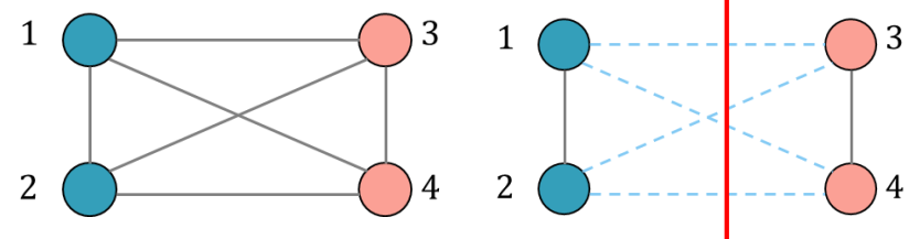
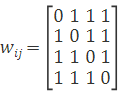
Through the connection relation, we can see that the adjacent matrix is
When vertex 1 and vertex 2 are assigned into one class and vertex 3 and vertex 4 are assigned into the other, \(\sigma_1=\sigma_2=1,\sigma_3=\sigma_4=-1\), then the above formula becomes:
Now the objective function is
The max number of cut is 4, which is consistent with the answers obtained through observation in the previous discussion.
Note that \(w_{ij}\) is an input constant and does not affect the calculation of the model, so the above formula can be simplified as:
where \(H\) is the Hamiltonian, \(w\) is the input adjacent matrix, decision variable \(\sigma_i\) represents the class of vertex \(i\) . This formula is an Ising model of the max-cut problem.
Modeling Code
Input the Matrix
import numpy as np
import kaiwu as kw

# Import the plotting library
import matplotlib.pyplot as plt

# invert input graph matrix
matrix = -np.array([
                [0, 1, 0, 1, 1, 0, 0, 1, 1, 0],
                [1, 0, 1, 0, 0, 1, 1, 1, 0, 0],
                [0, 1, 0, 1, 1, 0, 0, 0, 1, 0],
                [1, 0, 1, 0, 0, 1, 1, 0 ,1, 0],
                [1, 0, 1, 0, 0, 1, 0, 1, 0, 1],
                [0, 1, 0, 1, 1, 0, 0, 0, 1, 1],
                [0, 1, 0, 1, 0, 0, 0, 0, 0, 1],
                [1, 1, 0, 0, 1, 0, 0, 0, 1, 0],
                [1, 0, 1, 1, 0, 1, 0, 1, 0, 1],
                [0, 0, 0, 0, 1, 1, 1, 0, 1, 0]])
Use CIM Simulator to Check Qubit Evolution
Check the qubit evolution of single CIM simulating by kaiwu.cim.simulator_coresimulator. The simulator takes inputs of CIM-Ising matrix, pump power, noise intensity, number of laps, lap step size, normalization factor, independent running times, and outputs the simulating quantities of qubit evolution. It is supposed to normalize the eigenvalue of the input matrix using kaiwu.cim.normalizer, before using this simulator.
matrix_n = kw.cim.normalizer(matrix, normalization=0.5)
output = kw.cim.simulator_core(
            matrix_n,
            c = 0,
            pump = 0.7,
            noise = 0.01,
            laps = 1000,
            dt = 0.1)
Calculate the Hamiltonian using the matrix that is not normalized.
h = kw.sampler.hamiltonian(matrix, output)
Plot the qubit evolution graph and Hamiltonian graph:
plt.figure(figsize=(10, 10))

# pulsing diagram
plt.subplot(211)
plt.plot(output, linewidth=1)
plt.title("Pulse Phase")
plt.ylabel("Phase")
plt.xlabel("T")

# Energy diagram
plt.subplot(212)
plt.plot(h, linewidth=1)
plt.title("Hamiltonian")
plt.ylabel("H")
plt.xlabel("T")

plt.show()

Check the optimal solution. Before checking the optimal solution, we need to binarize the output data of simulator kaiwu.cim.simulator_core, using kaiwu.sampler.binarizer. For kaiwu.sampler.binarizer, in this example, we only enter the first parameter to indicate the input solution set, and leave the remaining parameters as default.
c_set = kw.sampler.binarizer(output)
Optimal solution sampling, kaiwu.sampler.optimal_sampler. The binary solution set is sorted by energy, with the frontmost solution having the lowest energy.
opt = kw.sampler.optimal_sampler(matrix, c_set, 0)
Take the optimal solution. opt =(the set of solutions, the set of energy), where the first index is
best = opt[0][0]
print(best)
Simulated Calculation
Perform Calculations with the CIM Simulator
For large-scale calculation, we use kaiwu.cim.simulator simulator, with inputs including Ising matrix, pump power, noise intensity, number of laps, lap step size, normalization factor, independent running times, and it outputs unique binary qubit values. Before applying this simulator, there is no need to use kaiwu.cim.normalizerto normalize the eigenvalue of the input matrix.
output = kw.cim.simulator(
            matrix,
            pump = 0.7,
            noise = 0.01,
            laps = 50,
            dt = 0.1,
            normalization = 0.3,
            iterations = 10)
Output Result
opt = kw.sampler.optimal_sampler(matrix, output, 0)
best = opt[0][0]
max_cut = (np.sum(-matrix)-np.dot(-matrix,best).dot(best))/4
print("The obtained max cut is "+str(max_cut)+".")