Parameter Precision#

When solving real-world problems, quantum hardware platforms impose strict limits on parameter precision. For example, the special-purpose quantum computer (SPQC) supports only the 8-bit integer range $[-128,127]$ , so the coefficient dynamic range must be carefully controlled during modeling to ensure computability. Although the Ising model is closer to the physical implementation, the QUBO model remains the preferred modeling form for combinatorial optimization because of its intuitive binary-variable representation and constraint-handling mechanism. This explains why, under 8-bit precision limits, we still need to model with QUBO before converting the model.

When building a QUBO model, users should pay special attention to two core steps. First, the model conversion process must ensure that the coefficients of the Ising matrix strictly fall within the hardware-supported dynamic range. Second, different problem characteristics require flexible precision adaptation strategies, such as dynamic range compression or variable splitting. This section introduces four reference approaches for reducing precision with Kaiwu SDK.

After studying this section, developers facing 8-bit hardware precision limits can make full use of the modeling advantages of QUBO models and ultimately convert them into Ising models that satisfy quantum-computing hardware requirements.

1. Background#

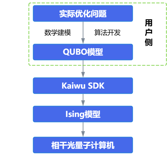
As shown above, a QUBO model is only a mathematical model, while an Ising model is closer to the physical implementation. Therefore, whether the user starts from a QUBO or Ising model, the final model solved on the real SPQC hardware is an Ising model. Thus, the 8-bit integer precision limit mentioned earlier applies to the Ising model, not to the QUBO model. To better check how the QUBO matrix should be limited so that the model satisfies the precision constraint, the following sections explain how to convert QUBO to an Ising model and why this limitation is needed.

1.1 Why reduce precision to 8 bit?#

In computer science and digital hardware design, an 8-bit integer is an integer stored with 8 binary bits. The 8-bit integer range discussed here is the signed integer range, with a minimum value of -128 and a maximum value of 127.

When using SPQC for computation, adopting the 8-bit integer range, namely $[-128,127]$ , as the parameter precision standard is not arbitrary. It is jointly determined by the physical characteristics of quantum hardware and computational requirements. At present, 8-bit precision provides the best balance between computational accuracy and hardware feasibility. As technology develops, this limit may be overcome through techniques such as error correction, but at the current stage, understanding and adapting to 8-bit precision is key to making full use of quantum advantages.

1.2 How to Convert QUBO to Ising?#

This section reviews how QUBO is converted into an Ising model to help explain how dynamic range checks constrain the QUBO matrix.

The Hamiltonian of the QUBO model is written as:

\mathcal{H}_{QUBO}= \sum_{i}{q_{ii}x_{i}} +\sum_{i\neq j}{q_{ij}x_{i}x_{j}}

where $x_i \in \{0,1\}$ is a binary variable, and $q_{ii}$ and $q_{ij}$ are the coefficients of the linear and quadratic terms, respectively. Because binary variables satisfy $x_i^2=x_i$ , the diagonal elements of a QUBO model can directly represent linear terms.

The variables of the Ising model are defined as spin variables $s_i \in \{-1,+1\}$ , and its Hamiltonian is:

\mathcal{H}_{Ising}= \sum_{i}{h_{i}s_{i}} +\sum_{i< j}{J_{ij}s_{i}s_{j}}

where $h_i$ is the local magnetic field and $J_{ij}$ is the coupling strength between spins.

To map the QUBO model to the Ising model, variable substitution is required. Let $s_{i} = 2x_{i}-1 \in \{1,-1\}$ . Substituting $x_i$ into the QUBO Hamiltonian gives:

\begin{aligned} \mathcal{H}_{Ising} =& \sum_{i}{q_{ii}\cdot \frac{s_{i}+1}{2}} +\sum_{i\neq j}{q_{ij}\cdot \frac{(s_{i}+1)(s_{j}+1)}{4}} \\ = &\sum_{i\neq j} \frac{q_{ij}}{4}s_{i}s_{j} +\sum_{i} \Big(\frac{q_{ii}}{2}+\frac{\sum_{k\neq i}{(q_{ik}+q_{ki})}}{4}\Big) s_{i} + \Big(\frac{\sum_{i} q_{ii}}{2} +\frac{\sum_{i\neq j}q_{ij}}{4}\Big) \end{aligned}

The coefficients of the Ising model are therefore:

\begin{aligned} J_{ij}&=\frac{q_{ij}}{4}\\ h_i&=\frac{q_{ii}}{2}+\frac{1}{4}\sum_{k\neq i}{(q_{ik}+q_{ki})} \end{aligned}

Here $h_i$ is the linear term. Because real SPQC hardware cannot directly solve Ising problems containing linear terms, an auxiliary variable must be added to convert them into quadratic terms. Therefore, when converting a QUBO matrix to an Ising matrix, the Ising matrix usually has one additional bit, that is, one additional variable. When the auxiliary variable takes values 1 and -1, it can correspond to the two solution sets before adding the auxiliary variable, respectively. Thus, the problem remains equivalent after adding the auxiliary variable. This is normal and users do not need to be concerned.

1.3 FAQ#

(1) The 8-bit integer range emphasized for the Ising matrix is not directly related to the specific values in the matrix. If all matrix elements are scaled by the same ratio and still fall within the 8-bit integer range, the computation requirements are also satisfied. For example, (1280, 1000) is equivalent to (128, 100);

(2) Why cannot the linear terms of an Ising matrix be placed on the diagonal elements?

QUBO variables satisfy $x^2 = x$ , so the diagonal elements of the matrix can represent linear terms. In the Ising model, $x^2 = 1$ , so this representation is not valid. Constant terms can usually be ignored during optimization, but they must be accumulated separately when computing the total energy. Record the constant term separately and add it when computing the final Hamiltonian.

Consider a simple QUBO model:

\begin{aligned} x^\top\left( \begin{array}{ll} 0 & 2\\ 1 & 1 \end{array}\right)x \end{aligned}

After the transformation, the Ising model is:

\begin{aligned} s^\top\left( \begin{array}{lll} 0 & 3/8 & 3/8\\ 3/8 & 0 & 5/8 \\ 3/8 & 5/8 & 0 \end{array} \right) s+3/2 \end{aligned}

2. Methods for Reducing Precision in Kaiwu SDK#

Kaiwu SDK provides four methods for reducing parameter precision: direct truncation (adjust_ising_matrix_precision), dynamic range compression (perform_precision_adaption_mutate), variable splitting (perform_precision_adaption_split), and the precision reduction decorator class (PrecisionReducer), which integrates adaptive truncation and variable splitting:

The direct truncation method is the simplest and most convenient, but extreme values may cause severe precision loss;
The dynamic range compression method can preserve the solution of the matrix while modifying the matrix, but the degree of precision reduction depends on the reducible space of the matrix itself;
The variable splitting method can modify the matrix to any precision, but the number of bits in the new matrix grows quickly as the required precision change increases.

2.1 Method 1: Direct truncation (`adjust_ising_matrix_precision`)#

Direct rounding is the simplest precision adjustment scheme. It linearly scales all matrix elements to the target bit width, such as the 8-bit integer range -128 to 127, and then rounds them to integers. This method can be implemented with the adjust_ising_matrix_precision or adjust_qubo_matrix_precision function.

As shown in the following table, adjust_ising_matrix_precision is a direct rounding function for adjusting the precision of an Ising matrix, while adjust_qubo_matrix_precision can convert a QUBO matrix to an Ising matrix, adjust the precision of the generated Ising matrix with direct rounding, and then output the matrix in the corresponding QUBO matrix form.

Item	`adjust_ising_matrix_precision`	`adjust_qubo_matrix_precision`
Input	Ising matrix	QUBO matrix
Method	Direct rounding	Direct rounding
Workflow	Ising matrix -> adjusted Ising matrix	QUBO matrix -> corresponding Ising matrix -> adjusted Ising matrix -> corresponding adjusted QUBO matrix
Output	Adjusted Ising matrix	Adjusted QUBO matrix

Example code:

ori_ising_mat1 = np.array(
    [
        [0, 0.22, 0.198],
        [0.22, 0, 0.197],
        [0.198, 0.197, 0],
    ]
)
ising_mat1 = kw.preprocess.adjust_ising_matrix_precision(ori_ising_mat1)
print("调整后矩阵:\n", ising_mat1)

The matrix comparison before and after adjustment is as follows:

\begin{bmatrix} 0 & 0.22 & 0.198 \\ 0.22 & 0 & 0.197 \\ 0.198 & 0.197 & 0 \end{bmatrix} \quad \rightarrow \quad \begin{bmatrix} 0 & 127 & 114 \\ 127 & 0 & 114 \\ 114 & 114 & 0 \end{bmatrix}

Note that this method works well for matrices whose elements have small differences, but when a matrix contains extreme values, direct rounding can cause severe precision loss. For example, for a matrix with an extreme value:

ori_ising_mat2 = np.array(
    [
        [0, 0.22, 0.198],
        [0.22, 0, 50],
        [0.198, 50, 0],
    ]
)
ising_mat2 = kw.preprocess.adjust_ising_matrix_precision(ori_ising_mat2)
print("极端值调整后矩阵:\n", ising_mat2)

The output is:

\begin{bmatrix} 0 & 0.22 & 0.198 \\ 0.22 & 0 & 50 \\ 0.198 & 50& 0 \end{bmatrix} \quad \rightarrow \quad \begin{bmatrix} 0 & 1 & 1 \\ 1 & 0 & 127 \\ 1 & 127 & 0 \end{bmatrix}

At this point, the small terms 0.22 and 0.198 are both compressed to 1, while the extreme value 50 is amplified to 127. However, the relative ratio between them is distorted by the precision upper bound (127) and the integer lower granularity (1), causing the solution to deviate from the true optimum. Therefore, direct rounding is recommended only for scenarios with a small dynamic range. For complex problems, dynamic range compression or variable splitting, introduced below, should be preferred.

2.2 Method 2: Dynamic range compression (`perform_precision_adaption_mutate`)#

Dynamic Range (DR) is a key metric for measuring the distribution of matrix coefficients. It applies to both QUBO matrices and Ising matrices. Reducing the dynamic range can reduce the parameter precision required by the original matrix.

The dynamic range is defined as:

DR(X):=log_2\left(\frac{\hat{D}(X)}{\check{D}(X)}\right)

where $X$ is the coefficient matrix, $\hat{D}(X) = \max_{i,j}|X_{ij}|$ is the maximum element distance of $X$ , and $\check{D}(X) = \min_{i,j}|X_{ij}|$ is the minimum element distance of $X$ .

Through matrix element rescaling and rounding, the original matrix $Q$ is mapped to the hardware-supported 8-bit integer range (-128 to 127) while preserving the optimal solution.

The specific steps are as follows. First, set the scaling factor to $\alpha$ and construct the transformation $Q' = \lfloor \alpha Q \rceil$ , where $\lfloor \cdot \rceil$ denotes rounding to the nearest integer.

The scaling factor must satisfy:

\alpha \leq \frac{127}{\hat{D}(Q)}

The transformed matrix then satisfies $Q'_{ij} \in [-128,127]$ .

Theoretical proof shows that when $\alpha$ satisfies:

\alpha > \frac{\Delta}{2\check{D}(Q)}

(where $\Delta$ is the minimum interval between adjacent distinguishable parameters), it can ensure $Q \subseteq Q'$ , meaning that the optimal solution of the original problem is included in the solution set of the new problem.

The dynamic range definition applies to both QUBO matrices and Ising matrices. Reducing the dynamic range can reduce the parameter precision required by the original matrix. Because the final computation is performed on the Ising matrix, Kaiwu SDK applies dynamic range reduction directly to the Ising matrix.

Kaiwu SDK mainly uses the perform_precision_adaption_mutate function for dynamic range compression. Take the following matrix as an example:

Q_0 = \begin{bmatrix} 0 & -20 & 0 & 40 & 1.1 \\ 0 & 0 & 12240 & 1 & 120 \\ 0 & 0 & 0 & 0 & -10240 \\ 0 & 0 & 0 & 0 & 2.05 \\ 0 & 0 & 0 & 0 & 0 \end{bmatrix}

After processing with perform_precision_adaption_mutate, the dynamic range is reduced from $DR(Q_0)=13.2$ to $DR(Q')=7.1$ while the optimal solution remains unchanged.

The detailed code is as follows:

np.random.seed(0)
mat0 = np.array(
    [
        [0, -20, 0, 40, 1.1],
        [0, 0, 12240, 1, 120],
        [0, 0, 0, 0, -10240],
        [0, 0, 0, 0, 2.05],
        [0, 0, 0, 0, 0],
    ]
)
mutated_mat = kw.preprocess.perform_precision_adaption_mutate(mat0)
print("调整后矩阵:\n", mutated_mat)

Running this program gives the adjusted matrix:

Q' = \begin{bmatrix} 0 & -2.05 & 0 & 2.05 & 0 \\ -2.05 & 0 & 4.1 & 0 & 0 \\ 0 & 4.1 & 0 & 0 & -2.05 \\ 2.05 & 0 & 0 & 0 & 2.05 \\ 0 & 0 & -2.05 & 2.05 & 0 \end{bmatrix}

2.3 Method 3: Variable splitting (`perform_precision_adaption_split`)#

Because current quantum computers store Ising coefficients as fixed-point numbers with only 8-bit precision, terms with a ratio between maximum and minimum coefficients greater than $2^{8}$ must be split if they have large coefficients. This is done by replacing bits in the original expression with multiple equivalent bits of equal value, where equality is enforced by constraint terms so that the coefficient of each term can be reduced. When the matrix parameter dynamic range exceeds the hardware-supported $2^{8}$ , variable splitting is required.

Let the objective function be:

f(\mathbf{x})=\sum_{i}q_i x_i+\sum_{i<j}q_{ij}x_i x_j

For terms satisfying $|q_{ij}| > 2^{16}$ , introduce the auxiliary variable $\mathbf{x'}$ to decompose them and construct the equivalent problem:

::

The splitting method converts $f(\mathbf{x})$ into:

\begin{aligned} &f(\mathbf{x}, \mathbf{x'})+M\sum_i (x_i - x_{i1})^2+M\sum_{i,j} (x_{ij}-x_{i(j+1)})= \\ &f(\mathbf{x}, \mathbf{x'})+M\sum_i (x_i + x_{i1} - 2x_ix_{i1})+M\sum_{i,j} (x_{ij} + x_{i(j+1)} - 2x_{ij}x_{i(j+1)}) \end{aligned}

For example, for $x_1+2x_2+200x_3$ , if the ratio between the maximum and minimum polynomial coefficients must not exceed 150, the polynomial is modified as:

x_1+2x_2+100x_3+100x_{31}+50(x_3-x_{31})^2=x_1+2x_2+100x_3+100x_{31}+50(x_3+x_{31}-2x_3x_{31})

mat = np.array(
    [
        [0, -15, 0, 40],
        [-15, 0, 0, 1],
        [0, 0, 0, 0],
        [40, 1, 0, 0],
    ]
)
splitted_ret, last_idx = kw.preprocess.perform_precision_adaption_split(mat, 4)
print(splitted_ret)

min_increment computes a default value of 1. The precision is set to 4 bits, with a range of $[-7,7]$ , meaning the absolute value should be less than 7. The program outputs the transformed matrix as follows:

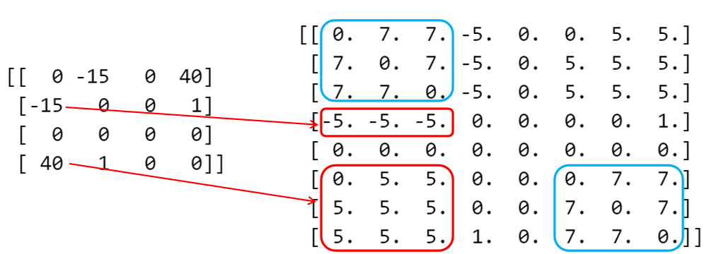
As shown in the figure, the red arrows indicate the correspondence before and after splitting, while the numbers in the blue boxes are penalty terms used to keep the values of the newly created variables consistent. By splitting variables this way, parameter precision can be reduced while preserving the solution of the original matrix. The precision reduction process is controlled by parameters such as param_bit, min_increment, penalty, and round_to_increment.

Here, the min_increment (minimum step size) parameter is used to reduce element precision while preserving the relative differences of the original data. This parameter makes matrix values integer multiples of min_increment; for example, when min_increment=0.5, elements can only be 0, 0.5, 1.0, and so on. Its default value is automatically computed as the minimum positive difference between matrix elements; for example, if the matrix contains 0.1 and 0.3, the default is min_increment=0.2.

The round_to_increment (rounding strategy) parameter is used to ensure that the sum of all elements is strictly equal to the original value when elements are adjusted. For example, when reduce_error is not enabled, 15 is split into 7.5+7.5, and approximate rounding would make them 8+8, causing the sum to deviate (15 -> 16). After reduce_error=True is enabled, the rounding direction of some elements is dynamically adjusted (7.5 -> 7 or 8), so the sum is strictly equal to the original value, such as 15 -> 7+8=15.

Demo code:

mat = np.array(
    [
        [0, -15, 0, 40],
        [-15, 0, 0, 1],
        [0, 0, 0, 0],
        [40, 1, 0, 0],
    ]
)
splitted_ret2, last_idx2 = kw.preprocess.perform_precision_adaption_split(
    mat, 4, min_increment=3, round_to_increment=True
)
print(splitted_ret2)

The result is:

\begin{bmatrix}0 & 21. & -6. & 0. & 3. & 12. \\ 21 & 0. & -9. & 0. & 12. & 12. \\ -6 & -9. & 0. & 0. & 0. & 0. \\ 0 & 0. & 0. & 0. & 0. & 0. \\ 3 & 12. & 0. & 0. & 0. & 21. \\ 12 & 12. & 0. & 0. & 21. & 0. \\ \end{bmatrix}

After obtaining the solution of the split matrix, use the restore_split_solution function to restore it to the solution of the original matrix.

original_solution = np.array([-1, 1, -1, -1])
split_solution = kw.preprocess.construct_split_solution(original_solution, last_idx)
org_sol = kw.preprocess.restore_split_solution(split_solution, last_idx)
print(org_sol)

The result is:

\begin{bmatrix} -1. & 1. & -1.& -1.\\ \end{bmatrix}

2.4 Method 4: Precision reduction decorator class (`PrecisionReducer`)#

The precision reduction decorator class (PrecisionReducer) is an intelligent precision adaptation scheme in Kaiwu SDK. Its core idea is to adapt the original matrix parameters to the hardware-supported precision range through a combined strategy of truncation and variable splitting. This scheme is implemented with the decorator pattern. Users can pass any optimizer as the base component, and PrecisionReducer automatically adjusts matrix precision during solving while ensuring solution feasibility. When submitting a problem to a quantum computer for solving, users can wrap CIMOptimizer with PrecisionReducer and then pass PrecisionReducer to Solver as the optimizer.

The decorator class works in two stages: truncation and variable splitting decision. After the user sets the target precision through the precision parameter, the decorator first computes the dynamic range of the matrix. If the dynamic range exceeds the hardware limit controlled by the target_bits parameter, it first attempts to reduce the dynamic range through a certain amount of adaptive truncation. If the precision requirement still cannot be met after truncation, variable splitting is triggered automatically to decompose large-coefficient terms into multiple equivalent variables and enforce their equivalence through penalty terms. The detailed example code is as follows:

kw.common.set_log_level("INFO")
matrix = -np.array(
    [
        [0.0, 1.23, 0.0, 1.0, 1.0],
        [1.23, 0.0, 0.0, 1.0, 1.0],
        [0.0, 0.0, 0.0, 1.0, 1.0],
        [1.0, 1.0, 1.0, 0.0, 1.0],
        [1.0, 1.0, 1.0, 1.0, 0.0],
    ]
)
base_optimizer = kw.classical.SimulatedAnnealingOptimizer(
    initial_temperature=100,
    alpha=0.99,
    cutoff_temperature=0.001,
    iterations_per_t=10,
    size_limit=5,
)
precision_optimizer = kw.preprocess.PrecisionReducer(base_optimizer, precision=8)
solution = precision_optimizer.solve(matrix)

The core parameter only_feasible_solution of the decorator class controls feasibility verification of solutions. When set to True, the decorator filters out all solutions that violate the splitting constraints, as judged by penalty terms, and raises an exception if all solutions are infeasible. When set to False, it allows infeasible solutions to be returned, which may contain inconsistent split variables.

For more usage details, refer directly to the kaiwu.preprocess package documentation: https://kaiwu-sdk-docs.qboson.com/zh/v1.2.0/source/modules/kaiwu.preprocess.html