Intelligent Scheduling, Efficient Empowerment: Unveiling the Path to Optimal Resource Allocation in Computing Power Networks#

算力网络，简单来说，就是将计算能力像水电一样进行输送的网络。想象一下，我们平时使用的手机、电脑等设备，都需要处理器来计算和运行各种程序。而算力网络就像是一个超级大的”处理器仓库”，它将分散在各地的计算资源整合起来，通过互联网进行优化分配，以满足不同用户和场景的计算需求。

举个例子，当我们观看高清视频、玩大型游戏或者进行复杂的数据分析时，这些操作都需要大量的计算能力。算力网络就像是一个智能的”电力系统”，能在短时间内为我们提供所需的计算资源，确保我们的使用体验流畅、高效。这样一来，我们就可以随时随地享受到强大的计算能力，而不用担心设备性能不足的问题。

Challenges Faced by Computing Power Networks#

Resource Allocation Efficiency: A computing power network needs to efficiently allocate computational resources to meet the diverse needs of different users and applications. This requires the network to monitor resource usage in real-time and dynamically adjust resource allocation strategies to avoid resource idleness or overload.
Network Latency: Quick response to computational tasks requires a low-latency network environment. A computing power network must address the latency issues in data transmission, especially when handling applications with high real-time requirements, such as autonomous driving.
Low Cost: Building and maintaining a computing power network requires significant financial investment, so it is necessary to minimize costs while ensuring performance.

Components of a Computing Power Network#

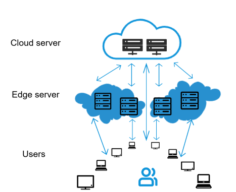
A computing power network mainly consists of three parts:

Edge Devices: These are various smart devices that are responsible for collecting data.
Edge Servers: Located near the devices, they are responsible for processing part of the data and alleviating the burden on cloud servers.
Cloud Servers: Located in data centers, they have powerful computing capabilities and are responsible for processing more complex data.

Problem Description#

Consider an optimization problem for the computing power network layout in a specific area. The area is divided into several adjacent square grids, and the computing power demand distribution data provides the computing power demand within each grid. The coordinate values in the data represent the center coordinates of the grid. To simplify the problem, the computing power demand points within each grid are unified to the grid center point (i.e., one grid corresponds to one demand point).

网格内的算力需求由端侧设备产生，端侧设备是连接到网络的终端设备，例如传感器、智能手机、工业机器人等。算力网络中的算力需求由边缘服务器和云端服务器满足。边缘服务器位于网络的”边缘”，通常靠近终端用户或设备。它们的任务是在离用户更近的地方处理数据，以提高响应速度和效率。边缘服务器可以更快地处理请求，因为它们距离用户更近。边缘服务器可以减轻核心云基础设施的负担，提高整体操作效率。云端服务器位于远离用户的数据中心，具有强大的计算和存储能力。当边缘服务器容量不足时，云端服务器可以作为补充。边缘服务器和云端服务器之间的协同作用可以优化整个系统的性能和可靠性。

Problem 1: In Problem 1, we only consider meeting the demand within the computing region using edge servers. Suppose we want to set up 2 edge servers within the grid area with computing power demand distribution, with each edge server having a coverage radius of 1. A QUBO model is required to determine at which points to place the edge servers to cover the maximum computing power demand.

Question 2: When the edge servers cannot meet the computational demand, upstream cloud servers will provide the necessary computing services. Now, a cloud server is added outside the grid area, and both end nodes and edge servers can choose to connect to the cloud node. When the computational demand received by the edge server exceeds its capacity, the excess demand will be directly allocated to the cloud server. The computational demand of each end node must be met and can only be served by one server, which can be either a cloud node or an edge server. Since edge servers have a resource capacity limit, assume that the available computational resource capacity of each edge server is 12, and the available computational resource capacity of the cloud server is infinite, meaning that the cloud server’s available computational resource capacity is not considered. Servers have a certain coverage radius, with the edge server’s coverage radius assumed to be 3, and the cloud server’s coverage radius is infinite, meaning that the cloud server’s coverage range is not considered.

Establishing edge servers typically incurs costs, which consist of fixed costs, computation costs, and transmission costs. The fixed cost is related to whether and where the edge server is established. The computation cost is proportional to the amount of requested computational resources, calculated as the unit computation cost multiplied by the computation amount. The unit computation cost for cloud servers is 1, while for edge servers, it is 2. Additionally, there is a transmission cost between the end node and the edge, from the edge to the cloud, and from the end to the cloud. The transmission cost is calculated by multiplying the computational demand by the transmission distance and the unit transmission cost. The transmission distance is calculated using the Euclidean distance, rounded to two decimal places, and calculated as a one-way distance (round-trip transmission is not considered). The unit transmission cost from the end to the edge and from the edge to the cloud is 1, while the unit transmission cost from the end to the cloud is 2.

To meet all the end-side computational demands within the area, establish a QUBO model to solve for the network layout that minimizes the overall cost, including the location and number of edge servers, and the connections between end-to-edge, edge-to-cloud, and end-to-cloud nodes.

The essence of the problem#

在算力网络布局优化问题中，表面上看，我们可能会联想到经典的资源调度问题或网络流优化问题，并尝试通过传统的贪心算法或动态规划方法来求解”如何在不同区域间分配资源以最小化成本”。这些方法或许能够帮助我们找到某一时刻的局部最优解，但这个问题的复杂性远超表面。我们不仅需要考虑每个计算节点的资源分配，还要全局性地优化整个网络的布局，保证每个资源都得到合理利用，并且在多个区域之间保持高效的计算和通信。

In-depth analysis#

The core of the computational network layout optimization problem is how to find an optimal resource allocation and node layout scheme across the entire network, similar to finding the optimal computational node layout and communication path combination in graph G. This is essentially a combinatorial optimization problem, requiring the selection of the optimal solution from all possible network layouts, and the number of these possible layouts is enormous. For example, if we have n potential edge server deployment locations and m computational task points, the combination of these locations and tasks will grow exponentially, with n^m possible layout combinations.

Obviously, a simple brute-force method is unrealistic because even for a moderately sized network, the number of combinations is astronomical, far beyond the capabilities of classical computers. Just like the path selection problem in the traveling salesman problem, we face a combinatorial challenge here, where every node and resource configuration in the network could affect the overall optimization result.

In other words, as the problem size increases, the time complexity of the algorithm grows non-polynomially, making it difficult to solve within a reasonable time. Therefore, the key to the problem is not how to locally optimize a single resource allocation, but how to globally optimize the entire computational network layout, finding the optimal layout path that minimizes overall computation costs. The complexity of this problem lies not only in the increase in computation but also in the need for multi-dimensional optimization to find a global optimal solution.

Reference model for the first question#

Restatement of the first question#

In a 4x4 grid, each grid represents an area with computational demand. Our goal is to determine in which grids to deploy edge computing nodes to maximize the covered user demand.

Symbol Definitions#

$R=1$ : Coverage radius of edge computing nodes
$P=2$ : Number of planned edge computing nodes to be deployed.
$\mathcal{L}_{u}$ : Set of user locations.
$\mathcal{L}_{e}$ : Set of candidate edge node locations.
$\text{demand}_{l} (l\in \mathcal{L}_{u})$ : Computational demand at grid $l$ .
$d_{ij}$ : Distance between grid $i$ and grid $j$ .
$\alpha_{ij}=\mathbb{1}_{d_{ij}\leq R}$ : Indicates whether the distance between grid $i$ and grid $j$ does not exceed the coverage radius $R$ of the edge node.

Decision Variables#

$x_{i}$ : A binary variable indicating whether to deploy an edge computing node in grid $i$ .
$z_{i}$ : A binary variable indicating whether grid $i$ is covered.

Objective Function#

Maximize the total covered computational demand:

$\max \sum_{i\in \mathcal{L}_{u}} {z_{i}\cdot \text{demand}_{i}}$

Constraints#

The coverage status of each user grid does not exceed the coverage status of the surrounding edge nodes:

$z_{i}\leq \sum_{j \in \mathcal{L}_{e}}{\alpha_{ij}\cdot x_{j}}, \forall i\in \mathcal{L}_{u}$
The total number of deployed edge computing nodes is equal to $P$ :

$\sum_{j\in \mathcal{L}_{e}} x_{j} = P$

Simplified Model (Inclusion-Exclusion Principle)#

When $P=2$ , we can simplify the model using the inclusion-exclusion principle:

$\max &\sum_{i\in \mathcal{L}_{u}} {\Big( \sum_{j \in \mathcal{L}_{e}}{\alpha_{ij}\cdot x_{j}} - \sum_{j,k \in \mathcal{L}_{e}}{\alpha_{ij} x_{j}}\cdot \alpha_{ik} x_{k}\Big)\text{demand}_{i}}\\ s.t. & \sum_{j\in \mathcal{L}_{e}} x_{j} = 2.$

Reference Model for Question 2#

Problem Overview#

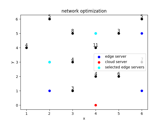
A 6×6 grid where each grid has a certain computational demand (only 11 grids have non-zero demand), and all computational demands need to be met.
There are 5 candidate locations for edge servers, each with limited computational capacity. When the computational requests received by an edge server exceed its capacity, the excess requests are sent to the cloud server.
One location hosts a cloud server, which has no capacity limit.
Users can connect to either the edge server or the cloud server (but only one); if the edge server’s capacity is insufficient, it can connect to the cloud server.
Minimize cost: fixed cost + variable cost (computational cost) + transmission cost (= unit cost * distance * transmission volume)

Symbol Definitions#

$C_{\text{edge}}$ : Edge server capacity.
$\text{c-fix-edge}_{j}$ : Fixed cost of establishing an edge computing node in grid $j$ .
$\text{c-var-cloud}$ : Unit computational cost at the cloud node.
$\text{c-var-edge}$ : Unit computational cost at the edge node.
$\text{c-tran}_{u,e}$ : Unit transmission cost from user side to edge side.
$\text{c-tran}_{u,c}$ : Unit transmission cost from user side to cloud side.
$\text{c-tran}_{e,c}$ : Unit transmission cost from edge side to cloud side.
$d_{ij}$ : Distance between grid $i$ and grid $j$ .
$d_{i}$ : The distance between grid $i$ and the cloud server.
$\alpha_{ij}=\mathbb{1}_{d_{ij} \leq R}$ : Whether the distance between grid $i$ and grid $j$ does not exceed the edge node coverage radius $R$

Intermediate Variables#

$y^{u,e}_{ij}$ : Whether the demand of grid $i$ is served by the edge server located at grid $j$
$y^{e,c}_{j}$ : Whether the edge server at grid $j$ is connected to the cloud server.
$y^{u,c}_{i}$ : Whether the demand of grid $i$ is served by the cloud server.
$u_{j} \in \mathbb{N}$ : The number of computational demands exceeding the capacity of edge server $j$ that are served by the cloud server.

Decision Variables#

$x_{\text{edge}, j}$ : Whether to open an edge server at location $j$ .

Mathematical Model#

Objective Function:

$\min \text{Cost}_{\text{fix}} + \text{Cost}_{\text{var}} + \text{Cost}_{\text{tran}}$

where

$\text{Cost}_{\text{fix}} = \sum_{j \in \mathcal{L}_{e}} \text{c-fix-edge}_{j} \cdot x_{\text{edge}, j}$

$\text{Cost}_{\text{var}} = &\text{c-var-cloud} \cdot \Big(\sum_{i \in \mathcal{L}_{u}} \text{demand}_{i} \cdot y^{u,c}_{i}\Big)\\ &+ \text{c-var-edge} \cdot \sum_{j \in \mathcal{L}_{e}} \sum_{i \in \mathcal{L}_{u}} \text{demand}_{i} \cdot y^{u,e}_{ij}\\ &+ (\text{c-var-cloud} - \text{c-var-edge}) \cdot \Big(\sum_{j \in \mathcal{L}_{e}} u_{j}\Big)$

$\text{Cost}_{\text{tran}} = &\text{c-tran}_{u,e} \cdot \sum_{i \in \mathcal{L}_{u}} \sum_{j \in \mathcal{L}_{e}} y^{u,e}_{ij} \cdot \text{demand}_{i} \cdot d_{ij}\\ &+ \text{c-tran}_{u,c} \cdot \sum_{i \in \mathcal{L}_{u}} y^{u,c}_{i} \cdot \text{demand}_{i} \cdot d_{i}\\ &+ \text{c-tran}_{e,c} \cdot \sum_{j \in \mathcal{L}_{e}} d_{j} \cdot u_{j}$

In this model, we express $u_{j}$ as

$u_{j} = y^{e,c}_{j} \cdot \Big(\sum_{i \in \mathcal{L}_{u}} \text{demand}_{i} \cdot y^{u,e}_{ij} - C_{\text{edge}}\Big)$

At the same time, we add constraints so that $y^{u,e}_{jk}$ will take the value of $1$ only when the computational demand received by edge server $j$ exceeds its capacity limit, otherwise it will be $0$ . Although the expression of $u_{j}$ contains quadratic terms, in this model, the cloud server has no capacity limit, and $u_{j}$ only appears in the objective function, not in the constraints, ensuring that no higher-order terms appear when converted to the QUBO model.

Constraints:

The computational demand points are allocated to either edge or cloud and are served by only one.

$\sum_{j \in \mathcal{L}_{e}}{y^{u,e}_{ij}} + y^{u,c}_{i} = 1, \forall i \in \mathcal{L}_{u}$
Coverage relationship, and only if the edge server is opened can it connect from the demand point.

$y^{u,e}_{ij} \leq \alpha_{ij} \cdot x_{\text{edge}, j}, \forall i \in \mathcal{L}_{u}, j \in \mathcal{L}_{e}$
The relationship between edge connection to the cloud and opening the edge server.

$y^{e,c}_{j} \leq x_{\text{edge}, j}, \forall j \in \mathcal{L}_{e}$
Only when the computational demand received by edge server $j$ exceeds its capacity limit, will $y^{u,e}_{jk}$ take the value of $1$ .

$y^{e,c}_{j} \cdot C_{\text{edge}} \leq \sum_{i \in \mathcal{L}_{u}}{\text{demand}_{i} \cdot \alpha_{ij} \cdot y^{u,e}_{ij}} \quad \text{(1)}$

$\sum_{i \in \mathcal{L}_{u}}{\text{demand}_{i} \cdot \alpha_{ij} \cdot y^{u,e}_{ij}} - C_{\text{edge}} \leq (\text{max-uj}[j] - C_{\text{edge}}) \cdot y^{e,c}_{j} \quad \text{(2)}$

where :math:text{max-uj}[j] is the upper bound of the computational demand received by edge server $j$ , which we set as

$\text{max-uj}[j] = \sum_{i \in \mathcal{L}_{u}}{\text{demand}_{i} \cdot \alpha_{ij}}$

Preprocessing#

For candidate locations of edge servers $j$ , if the computational demand they receive is always less than the edge server capacity limit, for example,

$\text{max-uj}[j] \leq C_{\text{edge}}$

When this is true, we can set $y^{e,c}_{j} = 0$ , and for this candidate location, inequalities (1) and (2) can be ignored to reduce the number of bits (relaxation variables).

Code for Question 1#

"""
JSP Problem Solving
"""
import math
import numpy as np
import kaiwu as kw


class JSPSolver:
    """Solver for JSP optimization problem."""

    def __init__(
            self,
            num_nodes: int = 2,
            coverage_range: float = 2.0,
            penalty: float = 100.0,
            num_slack_bins: int = 1,
    ) -> None:
        """Initialize JSPSolver parameters.

        Args:
            num_nodes: Number of edge nodes to be selected.

            coverage_range: Node coverage threshold.

            penalty: penalty coefficient.

            num_slack_bins: Slack binary digits, used to override constraints.
        """
        self.num_nodes = num_nodes
        self.coverage_range = coverage_range
        self.penalty = penalty
        self.num_slack_bins = num_slack_bins

        # Data containers
        self.demand = {}
        self.locations = []
        self.distances = {}
        self.coverage = {}
        self.dimension = 0

        # QUBO model
        self.model = None

    def prepare_data(self, demand_data):
        """prepare demand, distance, and coverage matrix data.

        Args:
            demand_data: dict, the key is the coordinate string 'i, j',
                        and the value corresponds to the calculation requirement.
        """
        self.demand = demand_data
        # Create a list containing all location coordinates
        self.locations = list(demand_data.keys())
        # Calculate the number of location coordinates
        self.dimension = int(math.sqrt(len(self.demand)))
        # Iterate through all location coordinates to calculate distances between pairs
        self.distances = {
            (i, j): np.linalg.norm(
                np.array([int(coord) for coord in i.split(',')])
                - np.array([int(coord) for coord in j.split(',')])
            )
            for i in self.locations
            for j in self.locations
        }
        # Initialize a dictionary to store the coverage relationship between locations
        self.coverage = {
            (i, j): int(dist <= self.coverage_range)
            for (i, j), dist in self.distances.items()
        }

    def prepare_model(self):
        """Building a Qubo Model
        """
        # Create binary variable arrays x and z to represent edge computing node locations
        # and demand coverage conditions
        var_x = kw.qubo.ndarray((self.dimension, self.dimension), 'x', kw.qubo.Binary)
        var_z = kw.qubo.ndarray((self.dimension, self.dimension), 'z', kw.qubo.Binary)
        # Initialize slack variables
        slack = kw.qubo.ndarray((self.dimension, self.dimension, self.num_slack_bins), 'slack', kw.qubo.Binary)
        # Define the objective function to minimize the total computing power demand
        obj = sum(
            self.demand[f'{i + 1},{j + 1}'] * var_z[i, j]
            for i in range(self.dimension)
            for j in range(self.dimension)
        )
        # Define the first constraint, ensuring the number of edge computing nodes equals P
        constr1 = (np.sum(var_x) - self.num_nodes) ** 2
        # Initialize the second constraint
        constr2 = 0
        # Iterate through all location coordinates to build the second constraint
        for i in range(self.dimension):
            for j in range(self.dimension):
                # For each location, the demand coverage z[i] should be less than or equal to
                # the total coverage provided by all edge computing nodes
                constr2 += (var_z[i, j] + sum(slack[i, j, _] * (2 ** i) for _ in range(self.num_slack_bins))
                            - sum(self.coverage[f'{i + 1},{j + 1}', f'{i1 + 1},{j1 + 1}'] * var_x[i1, j1]
                                  for i1 in range(self.dimension) for j1 in range(self.dimension))) ** 2

        self.model = kw.qubo.QuboModel()
        self.model.set_objective(-obj)
        self.model.add_constraint(constr1, name='c1', penalty=self.penalty)
        self.model.add_constraint(constr2, name='c2', penalty=self.penalty)

    def solve(self):
        """Solving the QUBO model.

        Returns:
            tuple: Result dictionary and Result dictionary.

            - dict: Result dictionary. The key is the variable name, and the value is the corresponding spin value.

            - float: qubo value.
        """
        # Perform the Simulated Annealing algorithm
        worker = kw.classical.SimulatedAnnealingOptimizer(
            initial_temperature=100000,
            alpha=0.99,
            cutoff_temperature=0.0001,
            iterations_per_t=100,
            rand_seed=10)
        _solver = kw.solver.SimpleSolver(worker)
        _sol_dict, _qubo_value = _solver.solve_qubo(self.model)
        return _sol_dict, float(_qubo_value)

    def recovery(self, sol_dict):
        """Verify whether the solution is feasible"""
        return self.model.verify_constraint(sol_dict)


if __name__ == "__main__":
    # Store computing power demand data in the DEM dictionary,
    # where the keys are location coordinates and the values are computing power demands
    demand_data = {'1,1': 38, '1,2': 22, '1,3': 65, '1,4': 56,
                   '2,1': 53, '2,2': 48, '2,3': 76, '2,4': 46,
                   '3,1': 56, '3,2': 36, '3,3': 7, '3,4': 29,
                   '4,1': 50, '4,2': 37, '4,3': 48, '4,4': 40}
    # Create an instance of the CIMSolver class
    solver = JSPSolver()

    # Prepare data
    solver.prepare_data(demand_data)

    # Prepare the QUBO model with a specified penalty coefficient lambda
    solver.prepare_model()

    # Use the Simulated Annealing algorithm to find the optimal solution
    best_sol_dict, qubo_value = solver.solve()

    # Recover the original problem solution from the QUBO solution and check its feasibility
    unsatisfied_count, result_dict = solver.recovery(best_sol_dict)
    if unsatisfied_count == 0:
        print("Find a feasible solution")
        print('Objective value:', -qubo_value)
    else:
        print("No feasible solution")

Code for Question 2#

"""Cloud-Edge-User Cost Minimization QUBO Model Solver."""
import math
from typing import Tuple
import numpy as np
import kaiwu as kw


class CloudEdgeUserSolver:
    """Solver for cloud-edge-user cost-minimization QUBO model."""

    def __init__(
            self,
            edge_capacity: int = 12,
            edge_radius: float = 3.0
    ) -> None:
        """Initialize core parameters and placeholders."""
        # capacities and radii
        self.edge_capacity = edge_capacity
        self.edge_radius = edge_radius

        # Service node configurations
        self.user_locations = ['1,1', '1,4', '2,6', '3,3', '3,5', '4,4', '5,5', '6,3', '6,6']
        self.edge_locations = ['6,1', '2,3', '4,5', '6,5']
        self.cloud_locations = ['4,0']

        # edge server costs
        self.fix_cost_edge = {'6,1': 60, '2,3': 42, '4,5': 46, '6,5': 54}

        # variable costs
        self.var_cost_cloud = 1
        self.var_cost_edge = 2

        # Unit transmission cost
        self.trans_cost_user_edge = 1
        self.trans_cost_user_cloud = 2
        self.trans_cost_edge_cloud = 1

        # Demand data
        self.demand = {
            '1,1': 7, '1,4': 4, '2,6': 5,
            '3,3': 9, '3,5': 8, '4,4': 11,
            '5,5': 1, '6,3': 7, '6,6': 5
        }

        # Precomputed data
        self.num_user = 0
        self.num_edge = 0
        self.num_cloud = 0
        self.distances = {}
        self.coverage = {}
        self.qubo_model = None

    def prepare_data(self):
        """Prepare data for QUBO model."""
        # initialize user demands
        loc_set_inner_full = ['1,1', '1,2', '1,3', '1,4', '1,5', '1,6',
                              '2,1', '2,2', '2,3', '2,4', '2,5', '2,6',
                              '3,1', '3,2', '3,3', '3,4', '3,5',
                              '4,1', '4,2', '4,3', '4,4', '4,5', '4,6',
                              '5,1', '5,2', '5,3', '5,4', '5,5', '5,6',
                              '6,1', '6,2', '6,3', '6,4', '6,5', '6,6']
        # all nodes
        loc_set = loc_set_inner_full + self.cloud_locations

        self.num_cloud = len(self.cloud_locations)
        self.num_edge = len(self.edge_locations)
        self.num_user = len(self.user_locations)

        # compute distances
        for i in loc_set:
            for j in loc_set:
                self.distances[(i, j)] = round(np.sqrt(
                    (int(i.split(',', maxsplit=1)[0]) - int(j.split(',', maxsplit=1)[0])) ** 2 + (
                            int(i.split(',', maxsplit=1)[1]) - int(j.split(',', maxsplit=1)[1])) ** 2), 2)

        # compute coverage relationships
        for i in loc_set:
            for j in loc_set:
                if self.distances[(i, j)] <= self.edge_radius:
                    self.coverage[(i, j)] = 1
                else:
                    self.coverage[(i, j)] = 0

    def prepare_model(
            self,
            eq_penalties: Tuple[float, float, float] = (1e4, 1e4, 1e4),
            ineq_penalties: Tuple[float, float] = (1e4, 1e4)
    ) -> None:
        """
        Build QUBO with 3 equality and 2 inequality constraints.
        """
        # compute the maximum demand for each edge
        max_ujk = []
        for j in self.edge_locations:
            max_ujk.append(sum(self.demand[i] * self.coverage[i, j] for i in self.user_locations))

        # initialize decision variables
        x_edge = kw.qubo.ndarray(self.num_edge, 'x_edge', kw.qubo.Binary)
        y_ij = kw.qubo.ndarray((self.num_user, self.num_edge), 'yij', kw.qubo.Binary)
        y_jk = kw.qubo.ndarray((self.num_edge, self.num_cloud), 'yjk', kw.qubo.Binary)
        y_ik = kw.qubo.ndarray((self.num_user, self.num_cloud), 'yik', kw.qubo.Binary)

        # for each edge, if the maximum demand does not exceed the edge's capacity, set the corresponding yjk to 0
        for j in range(self.num_edge):
            if max_ujk[j] <= self.edge_capacity:
                y_jk[j][0] = 0

        # initialize ujk related variables
        u_jk = np.zeros(shape=(self.num_edge, self.num_cloud), dtype=kw.qubo.QuboExpression)
        ujk_residual = np.zeros(shape=self.num_edge, dtype=kw.qubo.QuboExpression)
        for j in range(self.num_edge):
            ujk_residual[j] = sum(
                self.demand[self.user_locations[i]] * y_ij[i][j] for i in range(self.num_user)) - self.edge_capacity
            for k in range(self.num_cloud):
                u_jk[j][k] = y_jk[j][k] * ujk_residual[j]
        # build objective
        obj = self._build_objective_components(u_jk, x_edge, y_ij, y_ik)
        # build equality constraint
        constraint1, constraint2, constraint3 = self._build_eq_constraint(x_edge, y_ij, y_ik, y_jk)
        # build inequality constraint
        ineq_qubo1, ineq_qubo2 = self._build_ineq_constraint(max_ujk, ujk_residual, y_ij, y_jk)

        # building the final model
        self.qubo_model = kw.qubo.QuboModel()
        self.qubo_model.set_objective(obj)
        self.qubo_model.add_constraint(constraint1, name='c1', penalty=eq_penalties[0])
        self.qubo_model.add_constraint(constraint2, name='c2', penalty=eq_penalties[1])
        self.qubo_model.add_constraint(constraint3, name='c3', penalty=eq_penalties[2])
        self.qubo_model.add_constraint(ineq_qubo1, name='c4', penalty=ineq_penalties[0])
        self.qubo_model.add_constraint(ineq_qubo2, name='c5', penalty=ineq_penalties[1])

    def _build_ineq_constraint(self, max_ujk, ujk_residual, y_ij, y_jk):
        # inequality constraint 1: after subtracting the edge's maximum capacity from demand,
        # the yjk constraint should hold
        ineq_constraint1 = []
        ineq_qubo1 = kw.qubo.QuboExpression()
        len_slack1 = math.ceil(math.log2(max(max_ujk) + 1))
        slack1 = kw.qubo.ndarray((self.num_edge, self.num_cloud, len_slack1), 'slack1', kw.qubo.Binary)
        for j in range(self.num_edge):
            ineq_constraint1.append([])
            for k in range(self.num_cloud):
                if y_jk[j][k] == 0:
                    ineq_constraint1[j].append(0)
                else:
                    ineq_constraint1[j].append(
                        ujk_residual[j] - (max_ujk[j] - self.edge_capacity) * y_jk[j][k])
                    ineq_qubo1 += (ineq_constraint1[j][k] + sum(
                        slack1[j][k][_] * (2 ** _) for _ in range(len_slack1))) ** 2
        # inequality constraint 2: the capacity of an edge should be greater than or equal to the demand
        ineq_qubo2 = kw.qubo.QuboExpression()
        ineq_constraint2 = []
        len_slack2 = math.ceil(math.log2(max(max_ujk) + 1))
        slack2 = kw.qubo.ndarray((self.num_edge, self.num_cloud, len_slack2), 'slack2', kw.qubo.Binary)
        for j in range(self.num_edge):
            ineq_constraint2.append([])
            for k in range(self.num_cloud):
                if y_jk[j][k] == 0:
                    ineq_constraint2[j].append(0)
                else:
                    ineq_constraint2[j].append(y_jk[j][k] * self.edge_capacity - sum(
                        self.demand[self.user_locations[i]] * y_ij[i][j] for i in range(self.num_user)))
                    ineq_qubo2 += (ineq_constraint2[j][k] + sum(
                        slack2[j][k][_] * (2 ** _) for _ in range(len_slack2))) ** 2
        return ineq_qubo1, ineq_qubo2

    def _build_eq_constraint(self, x_edge, y_ij, y_ik, y_jk):
        # constraint 1: ensure that each user's service demand is assigned to only one location (either edge or cloud)
        constraint1 = 0
        for i in range(self.num_user):
            constraint1 += (sum(y_ij[i][j] for j in range(self.num_edge)) + sum(
                y_ik[i][k] for k in range(self.num_cloud)) - 1) ** 2
        # constraint 2: initialize constraint expression
        constraint2 = 0
        for i in range(self.num_user):
            for j in range(self.num_edge):
                if self.coverage[(self.user_locations[i], self.edge_locations[j])] == 0:
                    y_ij[i][j] = 0
                else:
                    constraint2 += y_ij[i][j] * (1 - x_edge[j])
        # constraint 3: ensure the relationship between yjk and x_edge
        constraint3 = 0
        for j in range(self.num_edge):
            for k in range(self.num_cloud):
                constraint3 += y_jk[j][k] * (1 - x_edge[j])
        return constraint1, constraint2, constraint3

    def _build_objective_components(self, u_jk, x_edge, y_ij, y_ik):
        # objective function
        c_fix = sum(self.fix_cost_edge[self.edge_locations[j]] * x_edge[j] for j in range(self.num_edge))
        c_var = self.var_cost_cloud * sum(sum(self.demand[self.user_locations[i]] * y_ik[i][k]
                                              for i in range(self.num_user)) for k in range(self.num_cloud))
        c_var += self.var_cost_edge * sum(
            sum(self.demand[self.user_locations[i]] * y_ij[i][j] for i in range(self.num_user))
            for j in range(self.num_edge))
        c_var += (self.var_cost_cloud - self.var_cost_edge) * sum(
            sum(u_jk[j][k] for j in range(self.num_edge)) for k
            in range(self.num_cloud))
        c_tran = self.trans_cost_user_edge * sum(sum(
            self.demand[self.user_locations[i]] * self.distances[(self.user_locations[i], self.edge_locations[j])] *
            y_ij[i][j] for i in range(self.num_user)) for j in range(self.num_edge))
        c_tran += self.trans_cost_user_cloud * sum(sum(
            self.demand[self.user_locations[i]] * self.distances[(self.user_locations[i], self.cloud_locations[k])] *
            y_ik[i][k] for i in range(self.num_user)) for k in range(self.num_cloud))
        c_tran += self.trans_cost_edge_cloud * sum(sum(
            self.distances[(self.edge_locations[j], self.cloud_locations[k])] * u_jk[j][k] for j in
            range(self.num_edge)) for k in range(self.num_cloud))
        return c_fix + c_tran + c_var

    def solve(
            self,
            max_iterations: int = 10,
            init_temp: float = 1e3,
            decay: float = 0.99,
            min_temp: float = 1e-4,
            iter_per_temp: int = 10
    ):
        """
        Perform simulated annealing.
        """
        best = math.inf
        for num in range(max_iterations):
            worker = kw.classical.SimulatedAnnealingOptimizer(
                initial_temperature=init_temp,
                alpha=decay,
                cutoff_temperature=min_temp,
                iterations_per_t=iter_per_temp
            )
            solver = kw.solver.SimpleSolver(worker)
            sol, val = solver.solve_qubo(self.qubo_model)
            feasible = self.recovery(sol)
            if feasible and val < best:
                best = val
                print(f"Iter {num}: best={val}")
        print(f"Optimal={best}")

    def recovery(self, sol_dict: dict) -> bool:
        """
        Validate solution via kaiwu.qubo.get_val interface.
        """
        unsatisfied_count, _ = self.qubo_model.verify_constraint(sol_dict)
        return not unsatisfied_count


if __name__ == "__main__":
    # create an instance of the solver class
    solver = CloudEdgeUserSolver()

    # prepare the data
    solver.prepare_data()

    # prepare the qubo model, set the penalty coefficient lambda
    solver.prepare_model()

    # use simulated annealing to find the optimal solution
    solver.solve()