智能调度，高效赋能：揭秘算力网络资源优化分配之道#

算力网络，简单来说，就是将计算能力像水电一样进行输送的网络。想象一下，我们平时使用的手机、电脑等设备，都需要处理器来计算和运行各种程序。而算力网络就像是一个超级大的“处理器仓库”，它将分散在各地的计算资源整合起来，通过互联网进行优化分配，以满足不同用户和场景的计算需求。

举个例子，当我们观看高清视频、玩大型游戏或者进行复杂的数据分析时，这些操作都需要大量的计算能力。算力网络就像是一个智能的“电力系统”，能在短时间内为我们提供所需的计算资源，确保我们的使用体验流畅、高效。这样一来，我们就可以随时随地享受到强大的计算能力，而不用担心设备性能不足的问题。

算力网络面临的挑战#

资源分配效率: 算力网络需要高效地分配计算资源以满足不同用户和应用的多样化需求。这要求网络能够实时监测资源使用情况，并动态调整资源分配策略，以避免资源闲置或过载。
网络延迟: 计算任务的快速响应需要低延迟的网络环境。算力网络必须解决数据在网络中传输的延迟问题，特别是在处理实时性要求高的应用时，如自动驾驶等。
成本要低: 搭建和维护算力网络需要投入大量资金，所以需要在保证性能的同时，尽量降低成本。

算力网络的组成部分#

算力网络主要由三个部分组成：

端侧设备: 也就是各种智能设备，它们负责收集数据。
边缘服务器: 位于设备附近，负责处理部分数据，并减轻云端服务器的负担。
云端服务器: 位于数据中心，拥有强大的计算能力，负责处理更复杂的数据。

赛题内容#

考虑一个特定区域的算力网络布局优化问题。将区域划分成若干相邻正方形网格，算力需求分布数据提供了各个网格内的算力需求。数据中的坐标值为所在网格的中心坐标，为简化问题，将各网格内的算力需求点统一到所在网格中心点（即可认为是一个网格对应一个需求点）。

网格内的算力需求由端侧设备产生，端侧设备是连接到网络的终端设备，例如传感器、智能手机、工业机器人等。算力网络中的算力需求由边缘服务器和云端服务器满足。边缘服务器位于网络的“边缘”，通常靠近终端用户或设备。它们的任务是在离用户更近的地方处理数据，以提高响应速度和效率。边缘服务器可以更快地处理请求，因为它们距离用户更近。边缘服务器可以减轻核心云基础设施的负担，提高整体操作效率。云端服务器位于远离用户的数据中心，具有强大的计算和存储能力。当边缘服务器容量不足时，云端服务器可以作为补充。边缘服务器和云端服务器之间的协同作用可以优化整个系统的性能和可靠性。

问题1: 在问题1中我们只考虑由边缘服务器满足计算区域内的需求。假设要在算力需求分布的网格区域内开设2个边缘服务器，每个边缘服务器的覆盖半径为1。要求建立QUBO模型，确定在哪些点放置边缘服务器可以覆盖最多的算力需求。

问题2: 当边缘服务器无法满足算力需求时，将由上游云端服务器提供计算服务。现在网格区域外部增设云端服务器，端侧和边缘服务器可以选择连接到云端节点，当边缘服务器接受的计算需求超过容量限制时，边缘服务器多余的需求将直接被分配到云端服务器。每个端侧节点的算力需求都必须被满足，且只能由一个服务器服务，这个计算节点可以是云端节点，也可以是边缘服务器。由于边缘服务器存在资源容量上限约束，假设每个边缘服务器的可用计算资源容量为12，云端服务器的可用计算资源容量为无穷大，即不考虑云端服务器的可用计算资源限制。服务器存在一定的覆盖半径，假设边缘服务器的覆盖半径为3，云端服务器的覆盖半径为无穷大，即不考虑云端服务器的覆盖范围。

开设边缘服务器通常需要成本，该成本由固定成本，计算成本和传输成本组成。其中固定成本与是否开设以及开设位置有关；计算成本与请求的计算资源量成正比，计算方法为：单位计算成本乘以计算量。云端服务器的单位计算量成本为1，边缘服务器的单位计算量成本为2。同时，从端侧到边侧、从边侧到云侧、从端侧到云侧之间的传输也存在传输成本，传输成本计算方式为：传输的算力需求量乘以传输距离乘以单位传输成本，其中传输距离的计算使用欧式距离保留两位小数，按照单边距离计算（不考虑往返传输）。从端侧到边侧以及从边侧到云侧的单位传输成本为1，从端侧到云侧的单位传输成本为2。

如果要满足区域内全部的端侧算力需求，建立QUBO模型，求解给出整体成本最小的算力网络布局，即边缘服务器的位置、数量，以及端侧到边侧、边侧到云侧和端侧到云侧节点之间的连接关系。

问题本质#

在算力网络布局优化问题中，表面上看，我们可能会联想到经典的资源调度问题或网络流优化问题，并尝试通过传统的贪心算法或动态规划方法来求解“如何在不同区域间分配资源以最小化成本”。这些方法或许能够帮助我们找到某一时刻的局部最优解，但这个问题的复杂性远超表面。我们不仅需要考虑每个计算节点的资源分配，还要全局性地优化整个网络的布局，保证每个资源都得到合理利用，并且在多个区域之间保持高效的计算和通信。

深入分析#

算力网络布局优化问题的核心是如何在整个网络中找到一种资源分配和节点布局的最优方案，类似于在图G上寻找最优的计算节点布局和通信路径组合。这实际上是一个组合优化问题，需要从所有可能的网络布局中挑选出最优解，而这些可能的布局数目是巨大的。例如，如果我们有n个潜在的边缘服务器部署位置和m个计算任务点，那么这些位置和任务的组合数量将以指数级别增长，即n^m种可能的布局方式。

显然，简单的穷举法是不现实的，因为即使是中等规模的网络，其组合数量也是天文数字，远远超出了经典计算机的处理能力。就像旅行商问题中的路径选择一样，我们在这里面临着一个排列组合的难题，网络中的每个节点和资源配置都可能影响整体的优化结果。

换句话说，随着问题规模的扩大，算法的时间复杂度呈现非多项式增长，难以在合理时间内求解。由此可见，问题的关键并不在于如何局部优化某一个资源配置，而在于如何全局性地优化整个算力网络的布局，找到那条能够最小化整体计算成本的最优布局路径。这个问题的复杂性不仅仅是计算量的增加，更在于需要在多维度上同时进行优化，寻找全局最优解。

第一问参考模型#

第一问重述#

在一个4x4的网格中，每个网格代表一定的计算需求区域。我们的目标是确定在哪些网格中部署边缘计算节点，以便最大化覆盖的用户需求。

符号定义#

$R=1$ : 边缘计算节点的覆盖半径。
$P=2$ : 计划部署的边缘计算节点个数。
$\mathcal{L}_{u}$ : 用户位置集合。
$\mathcal{L}_{e}$ : 候选边缘节点位置集合。
$\text{demand}_{l} (l\in \mathcal{L}_{u})$ : 位于网格 $l$ 处的算力需求量。
$d_{ij}$ : 网格 $i$ 和 $j$ 之间的距离。
$\alpha_{ij}=\mathbb{1}_{d_{ij}\leq R}$ : 网格 $i$ 和网格 $j$ 之间的距离是否不超过边缘节点覆盖半径 $R$ 。

决策变量#

$x_{i}$ : 一个二进制变量，表示是否在网格 $i$ 部署边缘计算节点。
$z_{i}$ : 一个二进制变量，表示网格 $i$ 是否被覆盖。

目标函数#

最大化总覆盖的计算需求量：

$\max \sum_{i\in \mathcal{L}_{u}} {z_{i}\cdot \text{demand}_{i}}$

约束条件#

每个用户网格的覆盖状态不超过其周围边缘节点的覆盖状态：

$z_{i}\leq \sum_{j \in \mathcal{L}_{e}}{\alpha_{ij}\cdot x_{j}}, \forall i\in \mathcal{L}_{u}$
部署的边缘计算节点总数等于 $P$ ：

$\sum_{j\in \mathcal{L}_{e}} x_{j} = P$

简化模型（容斥原理）#

当 $P=2$ 时，我们可以使用容斥原理来简化模型：

$\max &\sum_{i\in \mathcal{L}_{u}} {\Big( \sum_{j \in \mathcal{L}_{e}}{\alpha_{ij}\cdot x_{j}} - \sum_{j,k \in \mathcal{L}_{e}}{\alpha_{ij} x_{j}}\cdot \alpha_{ik} x_{k}\Big)\text{demand}_{i}}\\ s.t. & \sum_{j\in \mathcal{L}_{e}} x_{j} = 2.$

第二问参考模型#

问题概述#

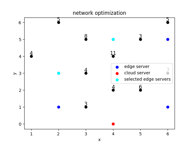
6×6的网格，每个网格内都有一定的计算需求(只有11个网格中的计算需求为非零值)，需要满足所有计算需求
5个开设边缘服务器的候选位置，边缘服务器具有计算容量限制; 当边缘服务器接收的计算请求超过容量时，将多出的计算请求发送给云端服务器
1个位置开设了云端服务器，云端服务器无容量限制
用户可以连接边缘服务器或者云端服务器(只能连一个); 边缘服务器容量不够可以连接云端服务器
最小化成本：固定成本 + 可变成本(计算成本) + 传输成本(=单位成本*距离*传输量)

符号定义#

$C_{\text{edge}}$ : 边侧服务器容量。
$\text{c-fix-edge}_{j}$ : 边缘计算节点开设在网格 $j$ 的固定成本。
$\text{c-var-cloud}$ : 云侧节点的单位计算量成本。
$\text{c-var-edge}$ : 边侧节点的单位计算量成本。
$\text{c-tran}_{u,e}$ : 从端侧到边侧的单位传输成本。
$\text{c-tran}_{u,c}$ : 从端侧到云侧的单位传输成本。
$\text{c-tran}_{e,c}$ : 从边侧到云侧的单位传输成本。
$d_{ij}$ : 网格 $i$ 和 $j$ 之间的距离。
$d_{i}$ : 网格 $i$ 和云端服务器之间的距离。
$\alpha_{ij}=\mathbb{1}_{d_{ij} \leq R}$ : 网格 $i$ 和网格 $j$ 之间的距离是否不超过边缘节点覆盖半径 $R$ 。

中间变量#

$y^{u,e}_{ij}$ : 网格 $i$ 的需求是否由位于网格 $j$ 的边侧服务器服务。
$y^{e,c}_{j}$ : 网格 $j$ 的边侧服务器是否连接云端服务器。
$y^{u,c}_{i}$ : 网格 $i$ 的需求是否由云端服务器服务。
$u_{j} \in \mathbb{N}$ : 超过边侧服务器 $j$ 的容量的计算需求中，由云端服务器服务的数量。

决策变量#

$x_{\text{edge}, j}$ : 是否在位置 $j$ 处开设边侧服务器。

数学模型#

目标函数:

$\min \text{Cost}_{\text{fix}} + \text{Cost}_{\text{var}} + \text{Cost}_{\text{tran}}$

其中

$\text{Cost}_{\text{fix}} = \sum_{j \in \mathcal{L}_{e}} \text{c-fix-edge}_{j} \cdot x_{\text{edge}, j}$

$\text{Cost}_{\text{var}} = &\text{c-var-cloud} \cdot \Big(\sum_{i \in \mathcal{L}_{u}} \text{demand}_{i} \cdot y^{u,c}_{i}\Big)\\ &+ \text{c-var-edge} \cdot \sum_{j \in \mathcal{L}_{e}} \sum_{i \in \mathcal{L}_{u}} \text{demand}_{i} \cdot y^{u,e}_{ij}\\ &+ (\text{c-var-cloud} - \text{c-var-edge}) \cdot \Big(\sum_{j \in \mathcal{L}_{e}} u_{j}\Big)$

$\text{Cost}_{\text{tran}} = &\text{c-tran}_{u,e} \cdot \sum_{i \in \mathcal{L}_{u}} \sum_{j \in \mathcal{L}_{e}} y^{u,e}_{ij} \cdot \text{demand}_{i} \cdot d_{ij}\\ &+ \text{c-tran}_{u,c} \cdot \sum_{i \in \mathcal{L}_{u}} y^{u,c}_{i} \cdot \text{demand}_{i} \cdot d_{i}\\ &+ \text{c-tran}_{e,c} \cdot \sum_{j \in \mathcal{L}_{e}} d_{j} \cdot u_{j}$

本模型中，我们将 $u_{j}$ 表示为

$u_{j} = y^{e,c}_{j} \cdot \Big(\sum_{i \in \mathcal{L}_{u}} \text{demand}_{i} \cdot y^{u,e}_{ij} - C_{\text{edge}}\Big)$

同时我们添加约束条件，使得当且仅当边侧服务器 $j$ 收到的计算需求超过其容量限制时， $y^{u,e}_{jk}$ 才会取值为 $1$ ，否则取值为 $0$ 。虽然 $u_{j}$ 的表达式中出现了二次项，但是本模型中云端服务器没有容量限制， $u_{j}$ 只出现在目标函数中，而不会出现在约束中，从而保证了转化成QUBO模型时不会出现高阶项。

约束条件:

算力需求点被分配到边侧或云侧，且只被一个服务

$\sum_{j \in \mathcal{L}_{e}}{y^{u,e}_{ij}} + y^{u,c}_{i} = 1, \forall i \in \mathcal{L}_{u}$
覆盖关系，且只有开了边侧才可以从需求点连接

$y^{u,e}_{ij} \leq \alpha_{ij} \cdot x_{\text{edge}, j}, \forall i \in \mathcal{L}_{u}, j \in \mathcal{L}_{e}$
边侧连接云侧和开启边侧的关系

$y^{e,c}_{j} \leq x_{\text{edge}, j}, \forall j \in \mathcal{L}_{e}$
当且仅当边侧服务器 $j$ 收到的计算需求超过其容量限制时， $y^{u,e}_{jk}$ 取值为 $1$

$y^{e,c}_{j} \cdot C_{\text{edge}} \leq \sum_{i \in \mathcal{L}_{u}}{\text{demand}_{i} \cdot \alpha_{ij} \cdot y^{u,e}_{ij}} \quad \text{(1)}$

$\sum_{i \in \mathcal{L}_{u}}{\text{demand}_{i} \cdot \alpha_{ij} \cdot y^{u,e}_{ij}} - C_{\text{edge}} \leq (\text{max-uj}[j] - C_{\text{edge}}) \cdot y^{e,c}_{j} \quad \text{(2)}$

其中 $\text{max-uj}[j]$ 为边侧服务器 $j$ 接收的计算需求的上界，这里我们令

$\text{max-uj}[j] = \sum_{i \in \mathcal{L}_{u}}{\text{demand}_{i} \cdot \alpha_{ij}}$

预处理#

对于边侧服务器候选位置 $j$ ，如果其接收的计算需求始终小于边侧服务器容量限制，例如

$\text{max-uj}[j] \leq C_{\text{edge}}$

成立时，可以令 $y^{e,c}_{j} = 0$ ，并且对于该候选位置，可以不考虑不等式约束 (1) 和 (2)，减少比特数（松弛变量数量）。

参考代码#

第一问代码#

import numpy as np
import math
import kaiwu as kw


class CIMSolver:
    def prepare_data(self):
        # Store computing power demand data in the DEM dictionary,
        # where the keys are location coordinates and the values are computing power demands
        DEM = {'1,1': 38, '1,2': 22, '1,3': 65, '1,4': 56, '2,1': 53, '2,2': 48, '2,3': 76, '2,4': 46, '3,1': 56,
               '3,2': 36, '3,3': 7, '3,4': 29, '4,1': 50, '4,2': 37, '4,3': 48, '4,4': 40}
        # Create a list containing all location coordinates
        LOC_SET = list(DEM.keys())

        # Initialize a dictionary to store distances between locations
        DIST = {}
        # Iterate through all location coordinates to calculate distances between pairs
        for i in LOC_SET:
            for j in LOC_SET:
                # Calculate Euclidean distance
                DIST[(i, j)] = np.sqrt((int(i.split(',')[0]) - int(j.split(',')[0])) ** 2 +
                                       (int(i.split(',')[1]) - int(j.split(',')[1])) ** 2)

        # Set the coverage radius of the edge computing nodes
        RANGE = 2

        # Set the target number of edge computing nodes
        P = 2

        # Initialize a dictionary to store the coverage relationship between locations
        ALPHA = {}
        for i in LOC_SET:
            for j in LOC_SET:
                # ALPHA is 1 if the distance is less than or equal to the coverage radius; otherwise, it is 0
                ALPHA[(i, j)] = 1 if DIST[(i, j)] <= RANGE else 0

        # Store the calculated results as instance variables
        self.ALPHA = ALPHA
        self.DIST = DIST
        self.DEM = DEM
        self.RANGE = RANGE
        self.P = P
        # Calculate the number of location coordinates
        self.d = int(math.sqrt(len(self.DEM)))

    # Prepare the QUBO model
    def prepare_model(self, lam):
        # Create binary variable arrays x and z to represent edge computing node locations
        # and demand coverage conditions
        self.x = kw.qubo.ndarray((self.d, self.d), 'x', kw.qubo.Binary)
        self.z = kw.qubo.ndarray((self.d, self.d), 'z', kw.qubo.Binary)
        # Initialize slack variables
        self.num_bin = 1
        self.slack = kw.qubo.ndarray((self.d, self.d, self.num_bin), 'slack', kw.qubo.Binary)

        # Set penalty coefficient
        self.lam = lam
        # Define the objective function to minimize the total computing power demand
        self.obj = sum(self.DEM[f'{i + 1},{j + 1}'] * self.z[i, j] for i in range(self.d) for j in range(self.d))
        # Define the first constraint, ensuring the number of edge computing nodes equals P
        self.constr1 = (np.sum(self.x) - self.P) ** 2
        # Initialize the second constraint
        self.constr2 = 0
        # Iterate through all location coordinates to build the second constraint
        for i in range(self.d):
            for j in range(self.d):
                # For each location, the demand coverage z[i] should be less than or equal to
                # the total coverage provided by all edge computing nodes
                self.constr2 += (self.z[i, j] + sum(self.slack[i, j, _] * (2 ** i) for _ in range(self.num_bin))
                                 - sum(self.ALPHA[f'{i + 1},{j + 1}', f'{i1 + 1},{j1 + 1}'] * self.x[i1, j1]
                                          for i1 in range(self.d) for j1 in range(self.d))) ** 2

        Q = self.lam * (self.constr1 + self.constr2) - self.obj
        self.qubo_model = kw.qubo.QuboModel()
        self.qubo_model.set_objective(Q)


    def sa(self, T_init=1000, alpha=0.99, T_min=0.0001, iterations_per_T=10):
        # Perform the Simulated Annealing algorithm
        worker = kw.classical.SimulatedAnnealingOptimizer(
            initial_temperature=T_init,
            alpha=alpha,
            cutoff_temperature=T_min,
            iterations_per_t=iterations_per_T)
        SimpleSolver = kw.solver.SimpleSolver(worker)
        sol_dict, self.qubo_val = SimpleSolver.solve_qubo(self.qubo_model)
        return sol_dict

    def recovery(self, sol_dict, option='inequality'):

        # Compute the value of the objective function
        obj_val = kw.qubo.get_val(self.obj, sol_dict)
        # Compute the value of the first constraint
        constr1_val = kw.qubo.get_val(self.constr1, sol_dict)

        # Check the second constraint based on the specified option
        if option == 'equality':
            constr2_flag = kw.qubo.get_val(self.constr2, sol_dict) == 0
        elif option == 'inequality':
            constr2_flag = True
            for i in range(self.d):
                for j in range(self.d):
                    # Check whether the demand coverage at each location satisfies the constraint
                    zij_val = kw.qubo.get_val(self.z[i, j], sol_dict)
                    x_total_val = kw.qubo.get_val(
                        sum(self.ALPHA[f'{i + 1},{j + 1}', f'{i1 + 1},{j1 + 1}'] * self.x[i1, j1]
                            for i1 in range(self.d) for j1 in range(self.d)), sol_dict)
                    if zij_val > x_total_val:
                        constr2_flag = False
                        break

        # Return the solution status based on the constraint satisfaction
        if constr1_val == 0 and constr2_flag:
            print('Find a feasible solution')
            print('Objective value:', obj_val)

def main():
    # Create an instance of the CIMSolver class
    solver = CIMSolver()

    # Prepare data
    solver.prepare_data()

    # Prepare the QUBO model with a specified penalty coefficient lambda
    lam = 100  # Set this value as needed
    solver.prepare_model(lam)

    # Use the Simulated Annealing algorithm to find the optimal solution
    best_solution = solver.sa(T_init=100000, alpha=0.99, T_min=0.0001, iterations_per_T=100)

    # Recover the original problem solution from the QUBO solution and check its feasibility
    solver.recovery(best_solution)


if __name__ == "__main__":
    main()

第二问代码#

import numpy as np
import kaiwu as kw
import math
#Define CIMSolver class
class CIMSolver:
# Initialize data
    def prepare_data(self, CAP_EDGE=10):
        # Initialize cloud server costs
        LOC_SET_OUTTER = ['4,0']
        self.C_FIX_CLOUD = {'4,0': 1500}
        self.LOC_SET_OUTTER = LOC_SET_OUTTER

        # Initialize edge server costs
        self.LOC_EDGE = ['6,1', '2,3', '4,5', '6,5']
        self.C_FIX_EDGE = {'6,1': 60, '2,3': 42, '4,5': 46, '6,5': 54}

        # Initialize variable costs
        C_VAR_CLOUD = 1
        C_VAR_EDGE = 2

        self.C_VAR_CLOUD = C_VAR_CLOUD
        self.C_VAR_EDGE = C_VAR_EDGE

        # Initialize user demands
        LOC_SET_INNER_full = ['1,1', '1,2', '1,3', '1,4', '1,5', '1,6', '2,1', '2,2', '2,3', '2,4', '2,5', '2,6', '3,1',
                              '3,2', '3,3', '3,4', '3,5', '4,1', '4,2', '4,3', '4,4', '4,5', '4,6', '5,1', '5,2',
                              '5,3', '5,4', '5,5', '5,6', '6,1', '6,2', '6,3',
                              '6,4', '6,5', '6,6']
        self.DEM = {'1,1': 7, '1,4': 4, '2,6': 5, '3,3': 9, '3,5': 8, '4,4': 11, '5,5': 1, '6,3': 7, '6,6': 5}
        self.LOC_SET_INNER = ['1,1', '1,4', '2,6', '3,3', '3,5', '4,4', '5,5', '6,3', '6,6']

        # Initialize transmission costs
        C_TRAN_ij = 1  # From end to edge
        C_TRAN_ik = 2  # From end to cloud
        C_TRAN_jk = 1  # From edge to cloud

        self.C_TRAN_ij = C_TRAN_ij
        self.C_TRAN_ik = C_TRAN_ik
        self.C_TRAN_jk = C_TRAN_jk

        # All nodes
        LOC_SET = LOC_SET_INNER_full + LOC_SET_OUTTER
        self.LOC_SET = LOC_SET

        self.num_cloud = len(self.LOC_SET_OUTTER)
        self.num_edge = len(self.LOC_EDGE)
        self.num_user = len(self.LOC_SET_INNER)

        # Compute distances
        DIST = {}
        for i in LOC_SET:
            for j in LOC_SET:
                DIST[(i, j)] = round(np.sqrt((int(i.split(',')[0]) - int(j.split(',')[0])) ** 2 + (
                        int(i.split(',')[1]) - int(j.split(',')[1])) ** 2), 2)
        self.DIST = DIST

        # Edge computing node coverage radius
        RANGE = 3
        self.RANGE = RANGE

        # Compute coverage relationships
        ALPHA = {}
        for i in LOC_SET:
            for j in LOC_SET:
                if DIST[(i, j)] <= RANGE:
                    ALPHA[(i, j)] = 1
                else:
                    ALPHA[(i, j)] = 0
        self.ALPHA = ALPHA
        self.CAP_EDGE = CAP_EDGE

    # Prepare model
    def prepare_model(self, lam_equ=None, lam=None):
        # Set penalty coefficients for equality constraints, default values are [10000, 10000, 10000]
        if lam_equ is None:
            lam_equ = [10000, 10000, 10000]
        if lam is None:
            lam = [10000, 10000]
        self.lam_equ = lam_equ

        # Set penalty coefficients for inequality constraints
        self.lam = lam

        # Compute the maximum demand for each edge
        self.max_ujk = []
        for j in self.LOC_EDGE:
            self.max_ujk.append(sum(self.DEM[i] * self.ALPHA[i, j] for i in self.LOC_SET_INNER))
        # print('self.max_ujk', self.max_ujk)

        # Initialize decision variables
        self.x_edge = kw.qubo.ndarray(self.num_edge, 'x_edge', kw.qubo.Binary)
        self.yij = kw.qubo.ndarray((self.num_user, self.num_edge), 'yij', kw.qubo.Binary)
        self.yjk = kw.qubo.ndarray((self.num_edge, self.num_cloud), 'yjk', kw.qubo.Binary)
        self.yik = kw.qubo.ndarray((self.num_user, self.num_cloud), 'yik', kw.qubo.Binary)

        # For each edge, if the maximum demand does not exceed the edge's capacity, set the corresponding yjk to 0
        for j in range(self.num_edge):
            if self.max_ujk[j] <= self.CAP_EDGE:
                self.yjk[j][0] = 0

        # Constraint 2: Initialize constraint expression
        self.constraint2 = 0
        for i in range(self.num_user):
            for j in range(self.num_edge):
                if self.ALPHA[(self.LOC_SET_INNER[i], self.LOC_EDGE[j])] == 0:
                    self.yij[i][j] = 0
                else:
                    self.constraint2 += self.yij[i][j] * (1 - self.x_edge[j])

        # Initialize ujk related variables
        self.ujk = np.zeros(shape=(self.num_edge, self.num_cloud), dtype=kw.qubo.QuboExpression)
        self.ujk_residual = np.zeros(shape=self.num_edge, dtype=kw.qubo.QuboExpression)
        for j in range(self.num_edge):
            self.ujk_residual[j] = sum(
                self.DEM[self.LOC_SET_INNER[i]] * self.yij[i][j] for i in range(self.num_user)) - self.CAP_EDGE
            for k in range(self.num_cloud):
                self.ujk[j][k] = self.yjk[j][k] * self.ujk_residual[j]

        # Objective function
        self.c_fix = sum(self.C_FIX_EDGE[self.LOC_EDGE[j]] * self.x_edge[j] for j in range(self.num_edge))

        self.c_var = self.C_VAR_CLOUD * sum(sum(self.DEM[self.LOC_SET_INNER[i]] * self.yik[i][k]
                                                for i in range(self.num_user)) for k in range(self.num_cloud))
        self.c_var += self.C_VAR_EDGE * sum(
            sum(self.DEM[self.LOC_SET_INNER[i]] * self.yij[i][j] for i in range(self.num_user))
            for j in range(self.num_edge))
        self.c_var += (self.C_VAR_CLOUD - self.C_VAR_EDGE) * sum(sum(self.ujk[j][k] for j in range(self.num_edge)) for k
                                                                 in range(self.num_cloud))

        self.c_tran = self.C_TRAN_ij * sum(
            sum(self.DEM[self.LOC_SET_INNER[i]] * self.DIST[(self.LOC_SET_INNER[i], self.LOC_EDGE[j])] * self.yij[i][j]
                for i in range(self.num_user)) for j in range(self.num_edge))
        self.c_tran += self.C_TRAN_ik * sum(sum(
            self.DEM[self.LOC_SET_INNER[i]] * self.DIST[(self.LOC_SET_INNER[i], self.LOC_SET_OUTTER[k])] * self.yik[i][
                k]
            for i in range(self.num_user)) for k in range(self.num_cloud))
        self.c_tran += self.C_TRAN_jk * sum(sum(self.DIST[(self.LOC_EDGE[j], self.LOC_SET_OUTTER[k])] * self.ujk[j][k]
                                                for j in range(self.num_edge)) for k in range(self.num_cloud))
        self.obj = self.c_fix + self.c_var + self.c_tran

        # Constraint 1: Ensure that each user's service demand is assigned to only one location (either edge or cloud)
        self.constraint1 = 0
        for i in range(self.num_user):
            self.constraint1 += (sum(self.yij[i][j] for j in range(self.num_edge))
                                 + sum(self.yik[i][k] for k in range(self.num_cloud)) - 1) ** 2

        # Inequality constraint 1: After subtracting the edge's maximum capacity from demand, the yjk constraint should hold
        self.ineq_constraint1 = []
        self.ineq_qubo1 = 0
        self.len_slack1 = math.ceil(math.log2(max(self.max_ujk) + 1))
        self.slack1 = kw.qubo.ndarray((self.num_edge, self.num_cloud, self.len_slack1), 'slack1', kw.qubo.Binary)

        for j in range(self.num_edge):
            self.ineq_constraint1.append([])
            for k in range(self.num_cloud):
                if self.yjk[j][k] == 0:
                    self.ineq_constraint1[j].append(0)
                else:
                    self.ineq_constraint1[j].append(
                        self.ujk_residual[j] - (self.max_ujk[j] - self.CAP_EDGE) * self.yjk[j][k])
                    self.ineq_qubo1 += (self.ineq_constraint1[j][k] + sum(
                        self.slack1[j][k][_] * (2 ** _) for _ in range(self.len_slack1))) ** 2

        # Inequality constraint 2: The capacity of an edge should be greater than or equal to the demand
        self.ineq_qubo2 = 0
        self.ineq_constraint2 = []
        self.len_slack2 = math.ceil(math.log2(max(self.max_ujk) + 1))
        self.slack2 = kw.qubo.ndarray((self.num_edge, self.num_cloud, self.len_slack2), 'slack2', kw.qubo.Binary)

        for j in range(self.num_edge):
            self.ineq_constraint2.append([])
            for k in range(self.num_cloud):
                if self.yjk[j][k] == 0:
                    self.ineq_constraint2[j].append(0)
                else:
                    self.ineq_constraint2[j].append(self.yjk[j][k] * self.CAP_EDGE -
                                                    sum(self.DEM[self.LOC_SET_INNER[i]] * self.yij[i][j] for i in
                                                        range(self.num_user)))
                    self.ineq_qubo2 += (self.ineq_constraint2[j][k] + sum(self.slack2[j][k][_] * (2 ** _)
                                                                          for _ in range(self.len_slack2))) ** 2

        # Constraint 3: Ensure the relationship between yjk and x_edge
        self.constraint3 = 0
        for j in range(self.num_edge):
            for k in range(self.num_cloud):
                self.constraint3 += self.yjk[j][k] * (1 - self.x_edge[j])

        # Building the final model
        self.model = self.obj
        self.model += self.lam_equ[0] * self.constraint1 + self.lam_equ[1] * self.constraint2 \
                      + self.lam_equ[2] * self.constraint3
        self.model += self.lam[0] * self.ineq_qubo1 + self.lam[1] * self.ineq_qubo2

        # Convert the model to an Ising model
        Q = self.model
        self.qubo_model = kw.qubo.QuboModel()
        self.qubo_model.set_objective(Q)


    def sa(self, max_iter, ss=None, T_init=1000, alpha=0.99, T_min=0.0001, iterations_per_T=10):
        """
        Perform the simulated annealing algorithm to find the optimal solution.

        Parameters:
        - max_iter: Maximum number of iterations
        - T_init: Initial temperature
        - alpha: Temperature decay factor
        - T_min: Minimum temperature
        - iter_per_T: Number of iterations per temperature level
        """
        iter = 0
        current_best = math.inf  # Initialize the current best solution to infinity
        opt_obj = 0  # Desired optimal objective value (can be adjusted depending on the specific problem)
        init_solution = None  # Initialize the solution

        while (iter < max_iter and current_best > opt_obj):
            print(f'Starting iteration {iter}, current best solution = {current_best}')
            # print('Current best solution = ', current_best)

            # Perform the simulated annealing algorithm
            worker = kw.classical.SimulatedAnnealingOptimizer(
                initial_temperature=T_init,
                alpha=alpha,
                cutoff_temperature=T_min,
                iterations_per_t=iterations_per_T)
            self.solver = kw.solver.SimpleSolver(worker)
            sol_dict, qubo_val = self.solver.solve_qubo(self.qubo_model)

                # Recover the solution and calculate the objective value
            flag, val_obj = self.recovery(sol_dict)
            if flag:
                # print('Feasible solution, objective value:', val_obj)
                current_best = min(current_best, val_obj)  # Update the current best solution
            iter += 1
        # print(self.recovery(opt[0][0]))
        print('Optimal solution:', current_best)

    def recovery(self, sol_dict):
        """
        Recover the optimal solution and calculate constraint violations and objective value.

        Parameters:
        - best: Optimal solution vector

        Returns:
        - (flag, val_obj): flag indicates if the solution is feasible, val_obj is the objective value or the number of constraint violations
        """
        self.val_eq1 = kw.qubo.get_val(self.constraint1, sol_dict)  # Calculate the value of constraint 1
        self.val_eq2 = kw.qubo.get_val(self.constraint2, sol_dict)  # Calculate the value of constraint 2
        self.val_eq3 = kw.qubo.get_val(self.constraint3, sol_dict)  # Calculate the value of constraint 3
        num_ineq_vio = 0  # Counter for inequality violations
        Flag = True  # Flag indicating if the solution is feasible

        # Check equality constraints
        if self.val_eq1 + self.val_eq2 + self.val_eq3:
            Flag = False

        # Check inequality constraint 1
        for j in range(self.num_edge):
            for k in range(self.num_cloud):
                if self.ineq_constraint1[j][k] != 0 and kw.qubo.get_val(self.ineq_constraint1[j][k], sol_dict) > 0:
                    Flag = False
                    num_ineq_vio += 1

        # Check inequality constraint 2
        for j in range(self.num_edge):
            for k in range(self.num_cloud):
                if self.ineq_constraint2[j][k] != 0 and kw.qubo.get_val(self.ineq_constraint2[j][k], sol_dict) > 0:
                    Flag = False
                    num_ineq_vio += 1

        # Return results: if the solution is feasible, return the objective value, otherwise return the number of inequality violations
        return (True, kw.qubo.get_val(self.obj, sol_dict)) if Flag else (False, num_ineq_vio)

def main():
    # Create an instance of the CIMSolver class
    solver = CIMSolver()

    # Prepare the data
    solver.prepare_data()

    # Prepare the QUBO model, set the penalty coefficient lambda
    solver.prepare_model()

    # Use simulated annealing to find the optimal solution
    max_iter = 100
    solver.sa(max_iter)

if __name__ == "__main__":
    main()

智能调度，高效赋能：揭秘算力网络资源优化分配之道

目录

智能调度，高效赋能：揭秘算力网络资源优化分配之道#

算力网络面临的挑战#

算力网络的组成部分#

赛题内容#

问题本质#

深入分析#

第一问参考模型#

第一问重述#

符号定义#

决策变量#

目标函数#

约束条件#

简化模型（容斥原理）#

第二问参考模型#

问题概述#

符号定义#

中间变量#

决策变量#

数学模型#

预处理#

参考代码#

第一问代码#

第二问代码#