Introduction Case Study - Genome Assembly#

What is Genome Assembly?#

Genome assembly is the process of using sequencing methods to generate sequence fragments (called reads) from the genome of the species to be studied. These fragments are then assembled based on overlapping regions between the reads. Initially, the fragments are joined into longer contiguous sequences (contigs), and then contigs are assembled into even longer scaffolds that may include gaps. By resolving errors and gaps in the scaffolds, we can map these scaffolds to chromosomes, ultimately producing a high-quality whole genome sequence. This process is crucial for studying species’ genome structures, functional gene discovery, metabolic network construction, and species evolution analysis.

With the advancements in sequencing technologies and the reduction in sequencing costs, we are now able to obtain large amounts of sequencing data in a short time. However, genome assembly is a complex process, particularly when dealing with the assembly of large and complex genomes of plants and animals, which require substantial computational resources. Therefore, efficiently analyzing and processing these data has become one of the most pressing issues in genomics and bioinformatics today.

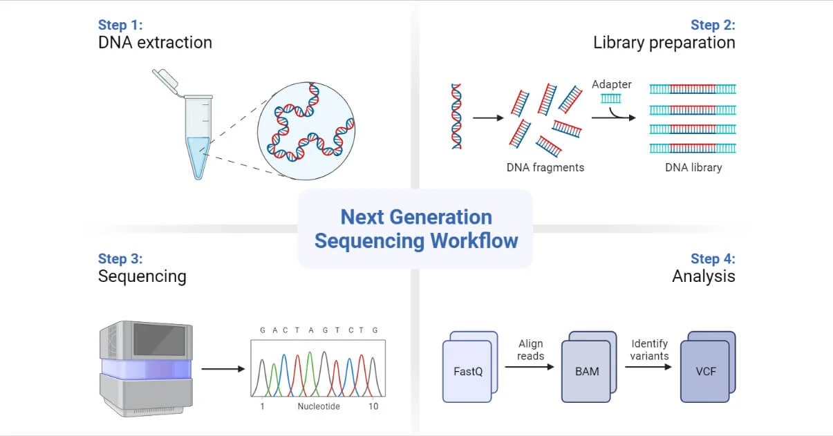
Figure 1: DNA Sequencing Flowchart (Source: Next-Generation Sequencing (NGS) - Definition, Types (microbenotes.com))

Common Genome Assembly Algorithms#

Genome assembly algorithms involve various methods, categorized into reference-based assembly and de novo assembly. The two most common de novo assembly strategies are De Bruijn graph-based assembly and Overlap-Layout-Consensus (OLC) assembly algorithms.

De Bruijn Graph:#

A De Bruijn graph is a directed graph consisting of nodes and edges. The graph requires that adjacent nodes differ by one base. By arranging the sequencing reads in k-mer fashion, the De Bruijn graph helps to assemble longer contigs. For example, if several reads overlap, they can be easily joined into a longer contig. The real scenario is more complex, but we typically retain the backbone path and assemble it into Contig1.

Overlap-Layout-Consensus (OLC):#

The OLC method first constructs an overlap graph, then converges it into contigs, and finally selects the most likely nucleotide sequence for each contig. The overlap graph represents sequences that share several identical bases at their ends. Multiple read fragments can form an overlap graph. The algorithm seeks the shortest contig sequence such that all the reads are subsets of this sequence, often implemented using a greedy algorithm.

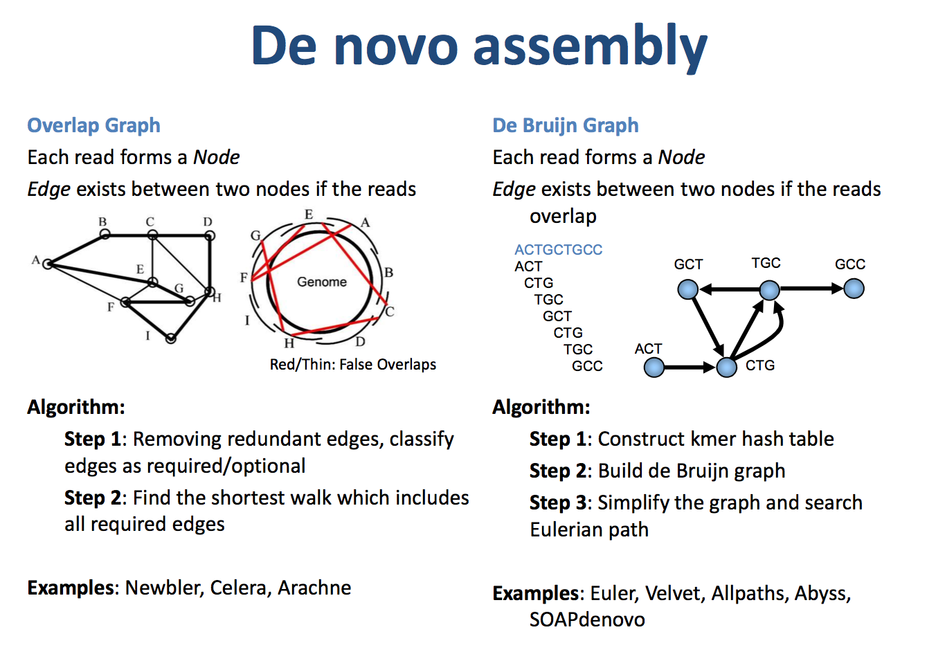
Figure 2: OLC (left) and DBG Algorithm Diagram (right) (Source: https://qinqianshan.com/bioinformatics/bin/olc-dbg/)

Applying Quantum Computing to Solve Genome Assembly Problems#

Problem Transformation#

High-quality genome assembly requires deep sequencing to meet the necessary depth. For a complete human genome assembly, a coverage of 30x or more is typically recommended. Using third-generation sequencing (e.g., PacBio and Oxford Nanopore) for human genome assembly, each read can span thousands to tens of thousands of bases. With 30x coverage, the required number of reads could range from several million to tens of millions. Assembling such a large number of reads for the overlap graph typically involves significant computational complexity and power requirements. Classical computing often uses methods such as overlap filtering and dynamic programming to reduce computational complexity, but assembling a high-quality genome still takes a lot of time. Here, we introduce quantum algorithms to accelerate this process.

The most critical step in the OLC algorithm is constructing the overlap graph to determine the positional relationships between different reads. This step can be transformed into a combinatorial optimization problem known as the Traveling Salesman Problem (TSP). In this case, different reads represent different city nodes, and the overlap length between reads serves as the weight between nodes. The objective is to sort all the reads based on their overlap length and try to assemble them into a single sequence with the longest overall overlap, as shown in Figure 3.

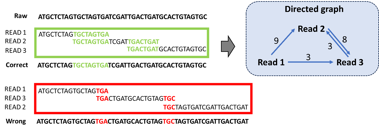
Figure 3: Sequencing Reads Assembly Transformed into Directed Graph Model

Modeling Steps#

1. Variable Definition#

In this model, we treat all reads as nodes, and the weight of the edges between the nodes is the overlap length between two reads that are connected in sequence. This forms a weighted directed graph. The goal is to find the longest overall overlap length for the reads sequence, which translates to finding the Hamiltonian cycle with the largest weight. The weighted directed graph is represented by an adjacency matrix: $\text{tspAdjMatrix}_{ij}$ , where the index elements represent the overlap length of $\text{Reads}_{i}$ followed by $\text{Reads}_{j}$ . If the overlap length is below a threshold or $i = j$ , then $\text{tspAdjMatrix}_{ij} = 0$ . The decision variable $\text{Reads}_{ij}$ takes values of $\{0, 1\}$ , where 1 indicates that $\text{Reads}_{i}$ is in the j-th position, otherwise 0.

To maximize the overlap length, the objective function can be written as:

$H_{\text{obj}} = \delta\sum_{\left( u,v \right) \in E}^{}{\text{tsp}\text{AdjMatrix}}_{u,v}(\sum_{j = 0}^{n - 1}{\text{Reads}_{u,j}\text{Reads}_{v,j + 1}} + \text{Reads}_{u,n - 1}\text{Reads}_{v,0})$

2. Constraints Handling#

Each read must and can only appear once in the sequence, $\sum_{j=1}^{n} \mathrm{{Reads\_Sort}}_{\mathrm{ij}} = 1$

Each position in the sequence must and can only be occupied by one read, $\sum_{i=1}^{n} \mathrm{{Reads\_Sort}}_{\mathrm{ij}} = 1$

The above two constraints can be written in QUBO form as follows:

$H_{seq\_ con} = \gamma\sum_{i = 0}^{N - 1}{(\sum_{j = 0}^{N - 1}{\text{Reads}_{\text{Sort}}}_{\text{ij}} - 1)}^{2}$

$H_{\text{node}\_ con} = \gamma\sum_{j = 0}^{N - 1}{(\sum_{i = 0}^{N - 1}{\text{Read}s_{\text{Sort}}}_{\text{ij}} - 1)}^{2}$

3. QUBO Model Construction#

Thus, from the above constraints, we can construct a model that traverses all the points in the path (also known as the Hamiltonian cycle):

$H = -H_{\mathrm{obj}} + H_{\mathrm{seq\_con}} + H_{\mathrm{node\_con}}$

The optimization goal is to minimize ( H )

4. Solver is used to solve QUBO Model directly with Kaiwu SDK#

import numpy as np
import kaiwu as kw
import random
import time

np.set_printoptions(linewidth=1000)
seed = 0


class DNAReconstruction:

    def __init__(self) -> None:
        pass

    def align(self, read1, read2, max_mismatch, cut_off):
        '''
        Overlap module, Read1 is the head and Read2 is the tail for alignment, returning the overlap length.
        read1 is the front gene fragment, read2 is the tail gene fragment, max_missmatch is the tolerance for mismatches, cut_off is the minimum overlap length threshold.
        read1 = 'AAATTTCCTTC'
        read2 = 'TTCCAGGT'
        mm = 0
        align(read1, read2, mm, 1)
        return 3
        align(read1, read2, mm, 3)
        return 0
        '''

        l1 = len(read1)
        l2 = len(read2)
        for shift in range(0, l1 - cut_off):
            mismatch = 0  # Number of mismatched bases
            r2i = 0
            for r1i in range(shift, l1):
                if read1[r1i] != read2[r2i]:
                    mismatch += 1  # Increment mismatch count
                if r2i < len(read2) - 1:
                    r2i += 1
                else:
                    break

                if mismatch > max_mismatch:  # If mismatches exceed tolerance, break out
                    break
            if mismatch <= max_mismatch:  # If mismatches are within tolerance, return overlap length
                return min(l1 - shift, l2)  # Return the overlap length as min(l1-shift, l2)
        return 0

    def aligncycle(self, read1, read2, max_mismatch, cut_off):

        l1 = len(read1)

        for shift in range(0, l1 - cut_off):
            mismatch = 0  # Number of mismatched bases
            r2i = 0
            for r1i in range(shift, l1):
                if read1[r1i] != read2[r2i]:
                    mismatch += 1  # Increment mismatch count
                if r2i < len(read2) - 1:
                    r2i += 1
                else:
                    break

                if mismatch > max_mismatch:  # If mismatches exceed tolerance, break out
                    break
            if mismatch <= max_mismatch:  # If mismatches are within tolerance, return overlap length
                return l1 - shift  # Return to the initial position
        return 0

    def shotGun(self, Gene_ref, reads_number, cut_off):
        # Given a gene sequence Gene_ref, replicate it reads_number times, connecting the ends, then randomly cut each loop in half
        self.reads = []  # Sequence reads
        self.cutpoint = []  # Cut points
        n = len(Gene_ref)

        for i in range(0, reads_number):  # Randomly cut the n-length gene sequence into two segments, resulting in 2n reads
            cut_1 = random.randint(0, len(Gene_ref) - 1)
            cut_2 = (cut_1 + round(len(Gene_ref) / 2) +
                     random.randint(-40, 40)) % n
            # Randomly cut the gene sequence at two points, making the segments approximately equal in length with a ±10% variation
            Gene_cut_1 = min(cut_1, cut_2)
            Gene_cut_2 = max(cut_1, cut_2)
            self.cutpoint.append(Gene_cut_1)
            self.cutpoint.append(Gene_cut_2)
            self.reads.append(Gene_ref[Gene_cut_1:Gene_cut_2 - 1])  # One segment
            self.reads.append(
                Gene_ref[Gene_cut_2 - 1:] + Gene_ref[0:Gene_cut_1])  # The other segment

    def merge_seq(self, DNAsort):
        # Consensus module, assemble DNA according to the sorting order. Given a sequence, return the reads assembled in that order.

        merge = self.reads[DNAsort[0]]  # Reconstruct the gene sequence
        n = len(self.reads)
        sum_overlap = 0  # Total overlap length
        r1i = 0
        r2i = 0

        # Connect gene fragments in the order of the solution, starting from the 0th and going to the n-1th
        while r2i < (n - 1):
            r2i += 1
            overlap = self.align(
                self.reads[DNAsort[r1i]], self.reads[DNAsort[r2i]], 0, 0)

            overlap1 = self.align(
                self.reads[DNAsort[r2i - 1]], self.reads[DNAsort[r2i]], 0, 0)

            sum_overlap = overlap1 + sum_overlap
            # If overlap length is greater than R2 length, R1 completely covers R2, skip fusion. R1 stays, and R2 moves to the next.
            if len(self.reads[DNAsort[r2i]]) > overlap:
                merge = merge + self.reads[DNAsort[r2i]][overlap:]
                r1i = r2i

        # Then connect the current longest tail with the 0th
        overlap = self.aligncycle(
            self.reads[DNAsort[n - 1 - r2i + r1i]], self.reads[DNAsort[0]], 0, 0)

        if overlap != 0:
            merge = merge[:-overlap]
        if len(self.reads[DNAsort[0]]) > overlap:
            sum_overlap = overlap + sum_overlap
        else:
            sum_overlap = len(self.reads[DNAsort[0]]) + sum_overlap
        return [merge, sum_overlap]

    def prepareModel(self, Gene_ref, reads_number, constraint, max_mismatch, cut_off):

        self.shotGun(Gene_ref, reads_number, cut_off)
        n = len(self.reads)
        # Convert DNA sequencing reads into a TSP adjacency matrix, where the edge weights are the overlaps, and the direction of the edge is row index → column index
        tspAdjMatrix = np.zeros((n, n))
        for r1 in range(0, n):
            for r2 in range(0, n):
                if r1 != r2:
                    tspAdjMatrix[r1][r2] = self.align(
                        self.reads[r1], self.reads[r2], max_mismatch, cut_off)

        # Create the QUBO variable matrix. The variable Reads_Sort(i,j) means that the i-th gene read is sorted in the j-th position
        self.Reads_Sort = kw.qubo.ndarray((n, n), "Reads_Sort", kw.qubo.Binary)

        w = tspAdjMatrix

        # Get the set of edges and non-edges
        edges = [(u, v) for u in range(n) for v in range(n) if w[u, v] != 0]

        # Read constraints: each read should belong to only one position
        sequence_cons = kw.qubo.quicksum(
            [(1 - kw.qubo.quicksum([self.Reads_Sort[v, j] for j in range(n)])) ** 2 for v in range(n)])

        # Position constraints: each position should have only one read
        node_cons = kw.qubo.quicksum(
            [(1 - kw.qubo.quicksum([self.Reads_Sort[v, j] for v in range(n)])) ** 2 for j in range(n)])

        # Hamiltonian cycle constraint, removing edge constraints
        self.ham_cycle = sequence_cons + node_cons

        # Total COST is the sum of overlap lengths; since the total length of DNA fragments should be minimized, COST should be maximized, so the negative sign is taken in the objective function
        self.path_cost = - kw.qubo.quicksum(
            [w[u, v] * (kw.qubo.quicksum([self.Reads_Sort[u, j] * self.Reads_Sort[v, j + 1]
                                          for j in range(n - 1)]) + self.Reads_Sort[u, n - 1] * self.Reads_Sort[v, 0])
             for u, v in edges])

        qubo_model = kw.qubo.QuboModel()
        obj = constraint * self.ham_cycle + self.path_cost
        qubo_model.set_objective(obj)

        self.qubo_model = qubo_model

    def printAnswer(self):
        # First restore the reference answer as an IS matrix, then add the spin term to get the reference answer's solution vector Answer_vec, and the reference answer provides other information
        self.Answer = np.argsort(self.cutpoint)  # Reference answer
        n = len(self.reads)  # Number of reads

        mat_answer = np.zeros((n, n), dtype=int)
        for i, x in enumerate(self.Answer):
            mat_answer[i, x] = 1
        return mat_answer


def main():
    dnaReconstruction = DNAReconstruction()
    Gene_ref = ('ATGGCTGCTAGGCTGTGCTGCCAACTGGATCCTGCGCGGGACGTCCTTTGTTTA'
                'CGTCCCGTCGGCGCTGAATCCTGCGGACGACCCTTCTCGGGGTCGCTTGGGACT'
                'CTCTCGTCCCCTTCTCCGTCTGCCGTTCCGACCGACCACGGGGCGCACCTCTCT')
    # Prepare the model, testing reads_number with 7, 8, 9, and 10
    # Duplicate the DNA sequence into reads_number copies, connect the ends,
    # and randomly cut each circle into two halves
    reads_number = 3
    # max_mismatch is the allowed mismatch in DNA alignment; exceeding it means the reads are not adjacent
    max_mismatch = 0
    # cut_off is the minimum overlap length threshold; if the overlap length between two reads
    # does not reach the threshold, it is set to 0
    cut_off = 3
    # The penalty coefficient for the Hamiltonian constraint in the final objective function
    constraint = 200

    '''
    Amplify the DNA sequence and randomly cut it into fragments using the shotgun method.
    Then sequence to obtain reads (this does not account for sequencing errors; fragments are directly used as reads).
    Store these reads as a weighted directed graph based on overlap length, and convert it into a TSP-like QUBO model.
    Based on the standard assembly order of the reference gene, provide the solution vector, Hamiltonian,
    and path length Hamiltonian for reference.
    '''
    dnaReconstruction.prepareModel(
        Gene_ref, reads_number, constraint, max_mismatch, cut_off)

    worker = kw.classical.SimulatedAnnealingOptimizer(initial_temperature=10000,
                                                      alpha=0.9,
                                                      cutoff_temperature=0.01,
                                                      iterations_per_t=200,
                                                      size_limit=100)
    solver = kw.solver.SimpleSolver(worker)
    sol_dict, qubo_val = solver.solve_qubo(dnaReconstruction.qubo_model)

    # Substitute the spin vector and obtain the result dictionary
    ham_val = kw.qubo.get_val(dnaReconstruction.ham_cycle, sol_dict)

    print('ham_cycle: {}'.format(ham_val))

    # Calculate the path length using path_cost
    path_val = kw.qubo.get_val(dnaReconstruction.path_cost, sol_dict)
    print('path_cost: {}'.format(path_val))


if __name__ == "__main__":
    main()

Comparison of Quantum Computing and Classical Methods#

We compared the solving time of the CIM real machine and traditional solvers (Simulated Annealing, Tabu Search) at different problem scales (reads of 7, 8, 9, and 10). The comparison shows that, for problems of the same scale, the solving time of CIM is much shorter than that of Simulated Annealing and Tabu Search (left figure). Moreover, as the problem scale increases, the CIM solving time becomes more stable compared to Simulated Annealing and Tabu Search (right).

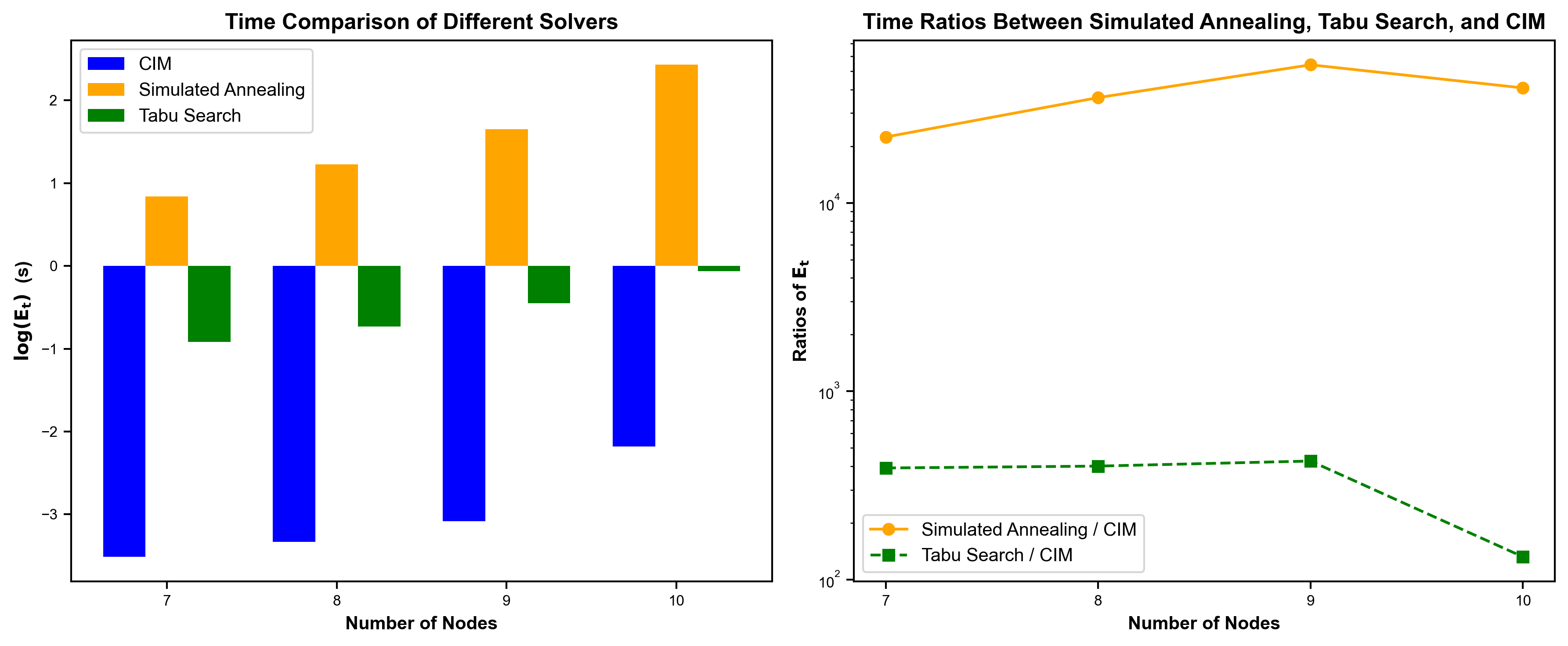
Figure 4: Comparison of Solving Time of CIM Real Machine and Traditional Solvers (Simulated Annealing, Tabu Search) at Different Problem Scales (reads of 7, 8, 9, 10)

For example, with 7 reads, we can see that the CIM real machine from the ‘TianGong Quantum Brain’ quickly reduces its Hamiltonian energy to find the optimal solution, compared to the SA algorithm.

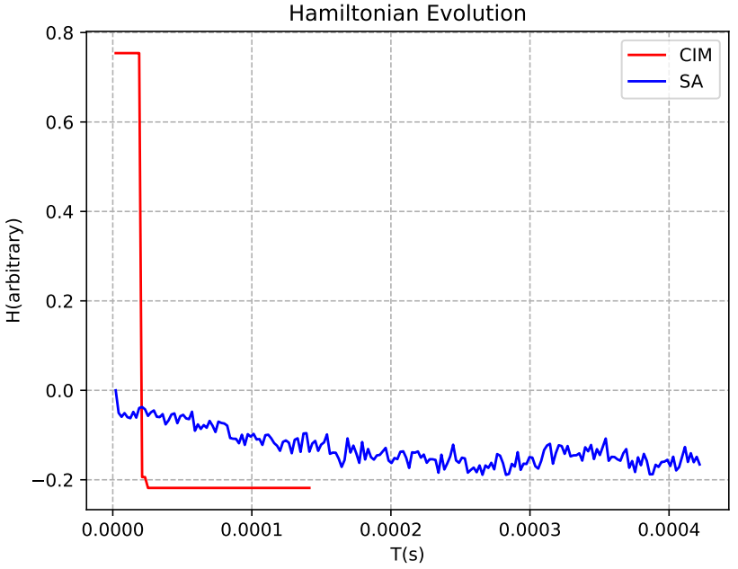
Figure 5: Hamiltonian Evolution for CIM (Red Line) and SA (Blue Line) with 7 Reads

Introduction Case Study - Genome Assembly

Contents