Case Study - Job Scheduling Problem (with Quantum Computing Comparison)#
🙋♀️🙋♂️What is the Job Scheduling Problem (JSP)?#
Task scheduling, though it sounds like a lofty field, is actually ubiquitous in our daily lives. You can think of it as a super-efficient secretary responsible for arranging tasks in a company. This secretary ensures that every task is handled at the right time, neither leaving employees idle nor allowing work to pile up. In computer science, task scheduling plays the same role, directing various tasks in a computer system to proceed in an orderly manner.
Imagine our computers or smartphones, which process thousands of tasks daily, such as opening apps, running programs, processing data, etc. Without a proper scheduling strategy, these tasks might collide with each other, causing the system to crash or slow down. The role of task scheduling is like that of a traffic officer, directing these tasks to proceed in an orderly fashion. It does this through carefully designed algorithms, such as priority scheduling, round-robin scheduling, and fair scheduling, ensuring that each task is processed at the appropriate time.
To put it simply, task scheduling is like the head chef in our kitchen. In the kitchen, there are tasks for washing vegetables, chopping them, and cooking. Each step has a different task. The head chef needs to arrange each person’s work based on the customer’s order, the availability of ingredients, and the chef’s specialties. Task scheduling works in a similar way; it decides which task should be executed first based on the urgency of the task, resource usage, and the overall system load.
In terms of logical rigor, researchers in the field of task scheduling need to consider many factors. For example, how to ensure that important tasks are prioritized without starving less important ones (i.e., tasks that are never executed for a long time); how to reasonably allocate resources like CPU and memory during concurrent multitasking to improve system throughput; and how to dynamically adjust the scheduling strategy during task execution to cope with a constantly changing system environment.
In short, task scheduling is a key area in computer science. It not only affects the performance of the electronic devices we use daily, but also impacts the efficiency and security of various fields such as data centers, cloud computing, and the Internet of Things. Through in-depth research into task scheduling, we can better utilize computer resources, improve work efficiency, and make our lives and work more convenient.
Application Case: Task Scheduling in Cloud Computing 🖧#
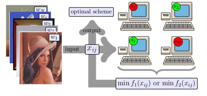
In a cloud computing environment, resource scheduling can be viewed as a JSP problem. Specifically, tasks in cloud computing can be seen as jobs, and servers as machines, with scheduling algorithms optimizing resource utilization and task completion time. Here is a basic example of cloud computing task scheduling:
Task Description: The customer submits a set of rendering tasks, each with a specific computational load.
Objective: Minimize the maximum completion time of all tasks.
Solution: By assigning tasks to appropriate servers and using quantum computing technology to optimize the scheduling plan, the goal of efficient resource utilization and early task completion can be achieved.
The basic components of JSP include:
Job: A task to be completed, each task consists of a single operation.
Machine: A resource that performs the tasks, with each machine able to handle only one task at a time.
Schedule: Assigning tasks to different machines and deciding the execution order of tasks on the machines (in this case, the execution order of tasks on machines does not affect the results).
To simplify the abstraction of the problem, the assumptions of the multi-machine task scheduling problem are summarized as follows:
The processing time required for each task is a fixed constant, depending only on the task itself.
The processing time required for each task is independent of the machine it is assigned to, assuming that all machines have the same task processing efficiency.
Each machine may have different idle start times, and cannot process tasks before these times.
Each task can only be assigned to one machine for execution.
A machine can process at most one task at a time.
After completing one task, a machine immediately proceeds to the next assigned task until all assigned tasks are completed.
All tasks must be completed.
Problem Definition 📖#
The running time of each task and the idle start time of each machine are integer values (e.g., multiples of the defined time precision). This facilitates converting the combinatorial optimization model into QUBO (Quadratic Unconstrained Binary Optimization) form to be compatible with specialized quantum computers.
To standardize the notation, the following definitions are made for the sets and data used in the multi-machine task scheduling problem:
Define the set of machines
, for example, M={Machine 1,Machine 2,…}, with the number of machines represented as
.
Define the set of tasks
, for example, N={Task 1, Task 2, …}, with the number of tasks represented as
.
Define the processing time required for task
as
.
Define the idle start time of machine
as
.
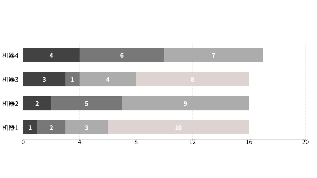
The following diagram shows an example of 4 machines handling 10 tasks. The vertical axis represents machines, and the horizontal axis represents time. The idle start times for each machine are 1, 2, 3, and 4. Each block with a number represents the duration of a task assigned to a machine. The allocation scheme shown minimizes the overall completion time and also provides an optimal solution for load balancing, ensuring that the completion times of all machines are as close as possible.
Mathematical Description of JSP and the QUBO Model#
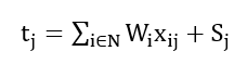
Define the binary variable ( X_{ij} ), which represents whether task ( i ) is assigned to machine ( j ). If task ( i ) is assigned to machine ( j ), then ( X_{ij} = 1 ); otherwise, ( X_{ij} = 0 ). Based on the previous definitions and assumptions, the task completion time on machine ( j ) can be expressed as
Next, the corresponding QUBO models are given for different objectives.
🕐Model 1: Minimize Overall Completion Time
For the first objective, which is to minimize overall completion time, the combinatorial optimization model is established as follows:
Define the variable as the overall latest completion time, which is the maximum of the completion times across all machines.
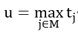
Objective Function

Constraints
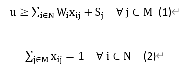
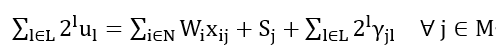
Constraint (1) states that the latest completion time ( u ) must be no less than the completion time ( t_j ) of any machine. Since the objective function is to minimize the latest completion time ( u ), the variable ( u ) will take the smallest value that satisfies (1), which is the completion time of the machine with the latest completion. Constraint (2) ensures that each task is executed by only one machine.
为了适配量子计算,需要将上面的组合优化模型转为QUBO形式,QUBO特点是所有决策变量为二值变量,目标是二次函数,且无约束条件。由于目标为整数,可用基于多个二值变量的二进制来表示:
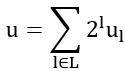
Here, ( X_{ij} ) represents a binary variable, which takes a value of 0 or 1. The set of binary digits required depends on the value of the data. Solving for the minimum value thus translates into solving for the binary values.
The next step is to convert the inequality constraint (1) into an equality constraint by adding slack variables. All slack variables are non-negative. Constraint (1) can be expressed as:
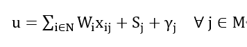
Since slack variables are integers, they are converted into binary. Constraint (1) can further be expressed as:
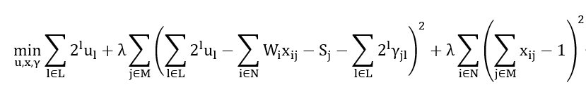
为了将等式约束化为目标函数的一部分从而满足QUBO形式,将等式约束改写为  的形式,然后将左侧取平方,乘以足够大的惩罚系数
  加入目标函数即可。这样当约束被满足,目标项中的相关项也就为0。目标最小化求解会倾向于让所有惩罚项为零,即所有约束被满足。这样,原模型就可以转化为以下QUBO模型:
🕐Model 2: Minimize the Completion Time Difference Across Machines (Load Balancing)
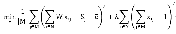
For the second objective, which is to minimize the completion time difference across machines, we minimize the variance of the completion times of all machines as the optimization goal, leading to the following combinatorial optimization model:
Objective Function
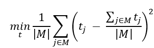
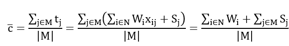
Note that the average completion time across machines is constant and independent of the allocation scheme, and is defined as  .
.
The approach to QUBOization is consistent with the previous model, so the QUBO model can be expressed as:
Model Code#
This code can be run and solved on the Kaiwu SDK.
import math
import numpy as np
import kaiwu as kw

# Output the number of unsatisfied constraints
def get_count_constr_not_met(solution_dict, print_detail=False):
    count_constr_not_met = 0  # Total number of unsatisfied constraints
    for t in SET_TASK:
        constr_value = kw.qubo.get_val(sum(x[(t, m)] for m in SET_MACHINE) - 1, solution_dict)
        if print_detail:
            print('constr_server_capacity', t, constr_value)
        if constr_value != 0:
            count_constr_not_met += 1
    return count_constr_not_met


# Output results
def result_summary(the_sol_dict):
    # Completion time for each machine
    max_complete_time = 0.0
    for m in SET_MACHINE:
        complete_time = kw.qubo.get_val(machine_endtime[m], the_sol_dict)
        if complete_time > max_complete_time:
            max_complete_time = complete_time
    return max_complete_time


if __name__ == '__main__':
    # Number of tasks
    N_TASK = 20
    # Number of machines
    N_MACHINE = 3

    seed = 12345
    np.random.seed(seed)

    # Index sets
    SET_TASK = {t for t in range(1, N_TASK + 1)}  # Tasks 1, 2, ..., N_TASK
    SET_MACHINE = {m for m in range(1, N_MACHINE + 1)}  # Machines 1, 2, ..., N_MACHINE

    # Model data
    DURATION = {t: np.random.randint(1, N_TASK + 1) for t in SET_TASK}  # Random task duration between 1 and 20
    START = {m: np.random.randint(1, N_MACHINE + 1) for m in SET_MACHINE}  # Random machine idle start time between 1 and 5

    # Penalty coefficient for constraints
    LAMBDA = 1000

    # Decision variables
    x = {(t, m): kw.qubo.Binary('x[' + str(t - 1) + '][' + str(m - 1) + ']') for t in SET_TASK for m in
         SET_MACHINE}  # Whether task i is assigned to machine j
    # QUBO objective function
    obj_function = 0.0
    # Variance term
    obj_function += sum(
        pow(
            START[m] + sum(DURATION[t] * x[(t, m)] for t in SET_TASK) -
            (sum(START[m] for m in SET_MACHINE) + sum(DURATION[t] for t in SET_TASK)) / N_MACHINE,
            2
        )
        for m in SET_MACHINE
    ) / N_MACHINE
    # Constraint term
    obj_function += LAMBDA * sum(pow(sum(x[(t, m)] for m in SET_MACHINE) - 1, 2) for t in SET_TASK)
    # End time for each machine
    machine_endtime = {
        m: START[m] + sum(DURATION[t] * x[(t, m)] for t in SET_TASK)
        for m in SET_MACHINE
    }

    qubo_model = kw.qubo.QuboModel()
    qubo_model.set_objective(obj_function)

    # Solve using simulated annealing
    max_iter = 40
    curr_iter = 0
    current_best = math.inf  # Initialize current best solution as infinity
    opt_obj = 0  # Desired optimal objective value (adjustable for specific problems)

    while (curr_iter < max_iter and current_best > opt_obj):
        print(f'Iteration {curr_iter} starts, current best solution = {current_best}')
        worker = kw.classical.SimulatedAnnealingOptimizer(
            initial_temperature=1000,
            alpha=0.99,
            cutoff_temperature=0.0001,
            iterations_per_t=10)
        solver = kw.solver.SimpleSolver(worker)
        # Get the optimal solution from simulated annealing output
        sol_dict, qubo_val = solver.solve_qubo(qubo_model)

        count_constr_not_met = get_count_constr_not_met(sol_dict, print_detail=False)
        if not count_constr_not_met:
            val_obj = result_summary(sol_dict)
            current_best = min(current_best, val_obj)  # Update current best solution

        curr_iter += 1
    print('Optimal solution:', current_best)
❇️Summary#
The Job Scheduling Problem (JSP) is a complex but practical optimization problem, widely applied in industries like manufacturing, project management, and cloud computing. Although solving JSP is challenging, advanced algorithms and technologies such as quantum computing can effectively optimize scheduling solutions, enhancing system efficiency and resource utilization.