Parameter Precision#

Parameter Precision conversion requirements#

QUBO is a commonly used modeling method in quantum computing, but physical machines execute on the Ising matrix. The QUBO model needs to be converted to the Ising model $\mathcal{H}=-\sum_{i,j}J_{ij}s_is_j-\mu\sum_ih_is_i$ for actual physical computation.

In actual computation, the coefficient bit width is limited by the hardware’s physical conditions and can only take a finite range.

1.The CIM machine only supports 8-bit INT space [-128, 127].

2.User modeling must ensure that the converted Ising matrix meets the requirements.

3.The provided conversion logic is for reference, and users can use more suitable methods based on their own matrices.

QUBO to Ising#

This section explains how to convert QUBO to Ising for better understanding of how dynamic range checking limits the QUBO matrix.

QUBO model

$\mathcal{H}= \sum_{i}{q_{ii}x_{i}} +\sum_{i\neq j}{q_{ij}x_{i}x_{j}}$

It needs to be converted into an Ising matrix before calculation. $s_{i} = 2x_{i}-1 \in \{1,-1\}$

$\mathcal{H} =& \sum_{i}{q_{ii}\cdot \frac{s_{i}+1}{2}} +\sum_{i\neq j}{q_{ij}\cdot \frac{(s_{i}+1)(s_{j}+1)}{4}} \\ = &\sum_{i\neq j} \frac{q_{ij}}{4}s_{i}s_{j} +\sum_{i} \Big(\frac{q_{ii}}{2}+\frac{\sum_{k\neq i}{(q_{ik}+q_{ki})}}{4}\Big) s_{i} + \Big(\frac{\sum_{i} q_{ii}}{2} +\frac{\sum_{i\neq j}q_{ij}}{4}\Big)$

The QUBO variable satisfies $x^2 = x$ , and the diagonal elements of the matrix can be used to express the linear terms. The Ising model $x^2 = 1$ cannot be expressed in this way.

The linear term in the above formula is added by adding an auxiliary variable $s'$ Transformed into quadratic terms, when the auxiliary variables take 1 and -1, they can respectively correspond to the two sets of solutions before adding the auxiliary variables. Therefore, adding auxiliary variables is equivalent to the original problem.

The constant terms are recorded separately and can be added when calculating the final Hamiltonian.

Example:

$x^\top\left( \begin{array}{ll} 0 & 2\\ 1 & 1 \end{array}\right)x$

After transformation, it is

$s^\top\left( \begin{array}{lll} 0 & 3/8 & 3/8\\ 3/8 & 0 & 5/8 \\ 3/8 & 5/8 & 0 \end{array} \right) s+3/2$

Methods for reducing precision in kaiwuSDK#

kaiwuSDK provides two methods to reduce parameter precision, perform_precision_adaption_mutate and perform_precision_adaption_split. The mutate method can keep the matrix solution unchanged while modifying the matrix, but the degree to which it can change the precision depends on the matrix’s own descending space The split method can modify the matrix to arbitrary precision, but the number of bits of the new matrix grows faster with the change in precision

perform_precision_adaption_mutate#

1 Dynamic Range#

1.1 QUBO matrix related definitions

Definition Q is QUBO matrix, and :math: ‘Q subseteq Q’ means that the optimal solution of Q is contained in the optimal solution of Q’

Definition $\lfloor Q \rceil$ is the round of each element of Q.

1.2 Definition of dynamic range

Definition $\hat{D}(X)$ is the maximum distance between elements of X

$\check{D}(X)$ is the minimum distance between elements of X

$DR(X):=log_2(\frac{\hat{D}(X)}{\check{D}(X)})$ is the dynamic range of X

Proposition $\hat{D}(Q)=1$ , then $\forall \alpha > 0, DR(\lfloor \alpha Q \rceil) \leq log_2(1+\alpha)$

By reducing the dynamic range, the parameter precision required by the original matrix can be reduced.

2. Examples#

import kaiwu as kw
import numpy as np

mat0 = np.array([[0, -20, 0, 40, 1.1],
                [0, 0, 12240, 1, 120],
                [0, 0, 0, 0, -10240],
                [0, 0, 0, 0, 2.05],
                [0, 0, 0, 0, 0]])
mutated_mat = kw.preprocess.perform_precision_adaption_mutate(mat0)
print(mutated_mat)

perform_precision_adaption_split#

1. Parameter Precision#

Because the current quantum computer stores QUBO coefficients as fixed-point numbers with only 8-bit accuracy, for polynomials with a ratio of maximum and minimum values exceeding $2^8$ , it is necessary to split the terms with large coefficients.

The method is to replace the bits in the original formula with multiple equivalent bits of equal value, and the equality condition is realized by the constraint term, so that the coefficient of each term can be reduced.

The QUBO expression, for example, is split by converting $f(\mathbf{x})$ to

$f(\mathbf{x}, \mathbf{x'})+M\sum_i (x_i - x_{i1})^2+M\sum_{i,j} (x_{ij}-x_{i(j+1)})^2= \\ f(\mathbf{x}, \mathbf{x'})+M\sum_i (x_i + x_{i1} - 2x_ix_{i1})+M\sum_{i,j} (x_{ij} + x_{i(j+1)} - 2x_{ij}x_{i(j+1)})$

For example, for $x_1+2x_2+200x_3$ , the ratio of the maximum and minimum values ofthe polynomial coefficients must not exceed 150, and the threshold is set to modify the polynomial to $x_1+2x_2+100x_3+100x_{31}+50(x_3-x_{31})^2=x_1+2x_2+100x_3+100x_{31}+50(x_3+x_{31}-2x_3x_{31})$

2. Examples#

import kaiwu as kw
import numpy as np

mat = np.array([[0, -15,0, 40],
                [-15,0, 0, 1],
                [0,  0, 0, 0],
                [40, 1, 0, 0]])
splitted_ret, last_idx = kw.preprocess.perform_precision_adaption_split(mat, 4)
print(splitted_ret)

min_increment computes a default value of 1. The precision is set to 4 bits in the range -7 to 7, which should definitely be less than 7.

The converted matrix of the program output is as follows:

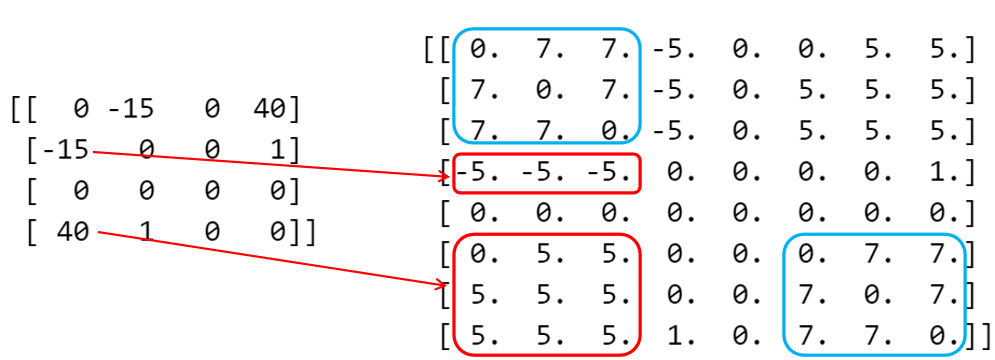
As shown in the figure, the red arrows indicate the corresponding relationships before and after the split. The number in the blue box is a penalty that limits the consistency of the value of the newly created variable. By splitting the variables in this way, the accuracy of the parameters can be reduced while maintaining the solution of the original matrix.

The precision reduction process is controlled by param_bit, min_increment, penalty, round_to_increment and other parameters.

Matrix values are integer multiples of min_increment, which defaults to the smallest positive difference between matrix elements

round_to_increment represents the process in which elements are adjusted so that the sum of the split elements equals the original value. For example, if 15 is divided into 7.5+7.5, it becomes 8+8 when approximately rounded. Set round_to_increment=True, 15 will be automatically split into 7+8

splitted_ret2, last_idx2 = kw.preprocess.perform_precision_adaption_split(mat, 4, min_increment=3, round_to_increment=True)
print(splitted_ret2)

The result is

[[ 0. 21. -6.  0.  3. 12.]
[21.  0. -9.  0. 12. 12.]
[-6. -9.  0.  0.  0.  0.]
[ 0.  0.  0.  0.  0.  0.]
[ 3. 12.  0.  0.  0. 21.]
[12. 12.  0.  0. 21.  0.]]

After solving the matrix whose precision meets the requirements after splitting, restore_splitted_solution can be used to restore it to the original matrix solution

worker = kw.cim.SimulatedCIMOptimizer(iterations=1000)
output = worker.solve(splitted_ret)
opt = kw.sampler.optimal_sampler(splitted_ret, output, bias=0, negtail_ff=False)
sol = opt[0][0]
org_sol = kw.preprocess.restore_splitted_solution(sol, last_idx)
print(org_sol)

The result is

[-1.  1. -1. -1.]

Parameter Precision

Contents

Parameter Precision#