Intelligent Scheduling, Efficient Empowerment: Unveiling the Path to Optimal Resource Allocation in Computing Power Networks

A computing power network, in simple terms, is a network that delivers computational power just like electricity or water. Imagine that the phones, computers, and other devices we use daily all require processors to compute and run various programs. The computing power network is like a massive ‘processor warehouse’ that consolidates scattered computing resources and optimizes their distribution via the internet to meet the computational needs of different users and scenarios.

For example, when we watch high-definition videos, play large-scale games, or perform complex data analysis, these operations require substantial computing power. The computing power network acts like an intelligent ‘power system’ that can quickly provide the necessary computational resources, ensuring a smooth and efficient user experience. This way, we can enjoy powerful computing capabilities anytime and anywhere without worrying about insufficient device performance.

Challenges Faced by Computing Power Networks

• Resource Allocation Efficiency: A computing power network needs to efficiently allocate computational resources to meet the diverse needs of different users and applications. This requires the network to monitor resource usage in real-time and dynamically adjust resource allocation strategies to avoid resource idleness or overload.

• Network Latency: Quick response to computational tasks requires a low-latency network environment. A computing power network must address the latency issues in data transmission, especially when handling applications with high real-time requirements, such as autonomous driving.

• Low Cost: Building and maintaining a computing power network requires significant financial investment, so it is necessary to minimize costs while ensuring performance.

Components of a Computing Power Network

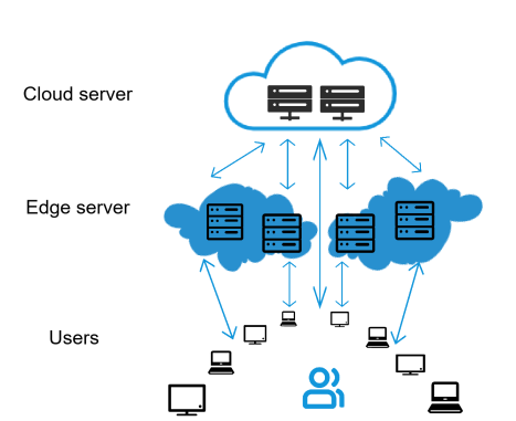
A computing power network mainly consists of three parts:

• Edge Devices: These are various smart devices that are responsible for collecting data.

• Edge Servers: Located near the devices, they are responsible for processing part of the data and alleviating the burden on cloud servers.

• Cloud Servers: Located in data centers, they have powerful computing capabilities and are responsible for processing more complex data.

Problem Description

Consider an optimization problem for the computing power network layout in a specific area. The area is divided into several adjacent square grids, and the computing power demand distribution data provides the computing power demand within each grid. The coordinate values in the data represent the center coordinates of the grid. To simplify the problem, the computing power demand points within each grid are unified to the grid center point (i.e., one grid corresponds to one demand point).

The computing power demand within the grid is generated by edge devices, which are terminal devices connected to the network, such as sensors, smartphones, and industrial robots. The computing power demand in the computing power network is met by edge servers and cloud servers. Edge servers are located at the ‘edge’ of the network, usually close to the end users or devices. Their task is to process data closer to the user to improve response speed and efficiency. Edge servers can process requests faster because they are closer to the users. Edge servers can also alleviate the burden on the core cloud infrastructure, improving overall operational efficiency. Cloud servers are located in data centers far from users and have powerful computing and storage capabilities. When the capacity of edge servers is insufficient, cloud servers can serve as a supplement. The collaboration between edge servers and cloud servers can optimize the performance and reliability of the entire system.

Problem 1: In Problem 1, we only consider meeting the demand within the computing region using edge servers. Suppose we want to set up 2 edge servers within the grid area with computing power demand distribution, with each edge server having a coverage radius of 1. A QUBO model is required to determine at which points to place the edge servers to cover the maximum computing power demand.

Question 2: When the edge servers cannot meet the computational demand, upstream cloud servers will provide the necessary computing services. Now, a cloud server is added outside the grid area, and both end nodes and edge servers can choose to connect to the cloud node. When the computational demand received by the edge server exceeds its capacity, the excess demand will be directly allocated to the cloud server. The computational demand of each end node must be met and can only be served by one server, which can be either a cloud node or an edge server. Since edge servers have a resource capacity limit, assume that the available computational resource capacity of each edge server is 12, and the available computational resource capacity of the cloud server is infinite, meaning that the cloud server’s available computational resource capacity is not considered. Servers have a certain coverage radius, with the edge server’s coverage radius assumed to be 3, and the cloud server’s coverage radius is infinite, meaning that the cloud server’s coverage range is not considered.

Establishing edge servers typically incurs costs, which consist of fixed costs, computation costs, and transmission costs. The fixed cost is related to whether and where the edge server is established. The computation cost is proportional to the amount of requested computational resources, calculated as the unit computation cost multiplied by the computation amount. The unit computation cost for cloud servers is 1, while for edge servers, it is 2. Additionally, there is a transmission cost between the end node and the edge, from the edge to the cloud, and from the end to the cloud. The transmission cost is calculated by multiplying the computational demand by the transmission distance and the unit transmission cost. The transmission distance is calculated using the Euclidean distance, rounded to two decimal places, and calculated as a one-way distance (round-trip transmission is not considered). The unit transmission cost from the end to the edge and from the edge to the cloud is 1, while the unit transmission cost from the end to the cloud is 2.

To meet all the end-side computational demands within the area, establish a QUBO model to solve for the network layout that minimizes the overall cost, including the location and number of edge servers, and the connections between end-to-edge, edge-to-cloud, and end-to-cloud nodes.

The essence of the problem

In the problem of computational network layout optimization, on the surface, we may think of classical resource scheduling or network flow optimization problems and try to solve ‘how to allocate resources among different areas to minimize costs’ using traditional greedy algorithms or dynamic programming methods. These methods might help us find a local optimal solution at a specific moment, but the complexity of this problem goes far beyond the surface. We not only need to consider the resource allocation of each computational node but also globally optimize the entire network layout, ensuring that each resource is reasonably utilized and that efficient computation and communication are maintained across multiple regions.

In-depth analysis

The core of the computational network layout optimization problem is how to find an optimal resource allocation and node layout scheme across the entire network, similar to finding the optimal computational node layout and communication path combination in graph G. This is essentially a combinatorial optimization problem, requiring the selection of the optimal solution from all possible network layouts, and the number of these possible layouts is enormous. For example, if we have n potential edge server deployment locations and m computational task points, the combination of these locations and tasks will grow exponentially, with n^m possible layout combinations.

Obviously, a simple brute-force method is unrealistic because even for a moderately sized network, the number of combinations is astronomical, far beyond the capabilities of classical computers. Just like the path selection problem in the traveling salesman problem, we face a combinatorial challenge here, where every node and resource configuration in the network could affect the overall optimization result.

In other words, as the problem size increases, the time complexity of the algorithm grows non-polynomially, making it difficult to solve within a reasonable time. Therefore, the key to the problem is not how to locally optimize a single resource allocation, but how to globally optimize the entire computational network layout, finding the optimal layout path that minimizes overall computation costs. The complexity of this problem lies not only in the increase in computation but also in the need for multi-dimensional optimization to find a global optimal solution.

Reference model for the first question

Restatement of the first question

In a 4x4 grid, each grid represents an area with computational demand. Our goal is to determine in which grids to deploy edge computing nodes to maximize the covered user demand.

Symbol Definitions

• : Coverage radius of edge computing nodes

• : Number of planned edge computing nodes to be deployed.

• : Set of user locations.

• : Set of candidate edge node locations.

• : Computational demand at grid .

• : Distance between grid and grid .

• : Indicates whether the distance between grid and grid does not exceed the coverage radius of the edge node.

Decision Variables

• : A binary variable indicating whether to deploy an edge computing node in grid .

• : A binary variable indicating whether grid is covered.

Objective Function

Maximize the total covered computational demand:

Constraints

• The coverage status of each user grid does not exceed the coverage status of the surrounding edge nodes:

  

• The total number of deployed edge computing nodes is equal to :

  

Simplified Model (Inclusion-Exclusion Principle)

When , we can simplify the model using the inclusion-exclusion principle:

Reference Model for Question 2

Problem Overview

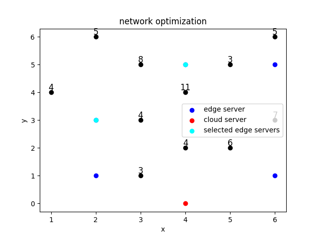
• A 6×6 grid where each grid has a certain computational demand (only 11 grids have non-zero demand), and all computational demands need to be met.

• There are 5 candidate locations for edge servers, each with limited computational capacity. When the computational requests received by an edge server exceed its capacity, the excess requests are sent to the cloud server.

• One location hosts a cloud server, which has no capacity limit.

• Users can connect to either the edge server or the cloud server (but only one); if the edge server’s capacity is insufficient, it can connect to the cloud server.

• Minimize cost: fixed cost + variable cost (computational cost) + transmission cost (= unit cost * distance * transmission volume)

Symbol Definitions

• : Edge server capacity.

• : Fixed cost of establishing an edge computing node in grid .

• : Unit computational cost at the cloud node.

• : Unit computational cost at the edge node.

• : Unit transmission cost from user side to edge side.

• : Unit transmission cost from user side to cloud side.

• : Unit transmission cost from edge side to cloud side.

• : Distance between grid and grid .

• : The distance between grid and the cloud server.

• : Whether the distance between grid and grid does not exceed the edge node coverage radius

Intermediate Variables

• : Whether the demand of grid is served by the edge server located at grid

• : Whether the edge server at grid is connected to the cloud server.

• : Whether the demand of grid is served by the cloud server.

• : The number of computational demands exceeding the capacity of edge server that are served by the cloud server.

Decision Variables

• : Whether to open an edge server at location .

Mathematical Model

Objective Function:

where

In this model, we express as

At the same time, we add constraints so that will take the value of only when the computational demand received by edge server exceeds its capacity limit, otherwise it will be . Although the expression of contains quadratic terms, in this model, the cloud server has no capacity limit, and only appears in the objective function, not in the constraints, ensuring that no higher-order terms appear when converted to the QUBO model.

Constraints:

• The computational demand points are allocated to either edge or cloud and are served by only one.

  

• Coverage relationship, and only if the edge server is opened can it connect from the demand point.

  

• The relationship between edge connection to the cloud and opening the edge server.

  

• Only when the computational demand received by edge server exceeds its capacity limit, will take the value of .

  

  

  where :math:text{max-uj}[j] is the upper bound of the computational demand received by edge server , which we set as

  

Preprocessing

For candidate locations of edge servers , if the computational demand they receive is always less than the edge server capacity limit, for example,

When this is true, we can set , and for this candidate location, inequalities (1) and (2) can be ignored to reduce the number of bits (relaxation variables).

Reference Code

Code for Question 1

import numpy as np
import math
import kaiwu as kw


class CIMSolver:
    def prepare_data(self):
        # Store computing power demand data in the DEM dictionary,
        # where the keys are location coordinates and the values are computing power demands
        DEM = {'1,1': 38, '1,2': 22, '1,3': 65, '1,4': 56, '2,1': 53, '2,2': 48, '2,3': 76, '2,4': 46, '3,1': 56,
               '3,2': 36, '3,3': 7, '3,4': 29, '4,1': 50, '4,2': 37, '4,3': 48, '4,4': 40}
        # Create a list containing all location coordinates
        LOC_SET = list(DEM.keys())

        # Initialize a dictionary to store distances between locations
        DIST = {}
        # Iterate through all location coordinates to calculate distances between pairs
        for i in LOC_SET:
            for j in LOC_SET:
                # Calculate Euclidean distance
                DIST[(i, j)] = np.sqrt((int(i.split(',')[0]) - int(j.split(',')[0])) ** 2 +
                                       (int(i.split(',')[1]) - int(j.split(',')[1])) ** 2)

        # Set the coverage radius of the edge computing nodes
        RANGE = 2

        # Set the target number of edge computing nodes
        P = 2

        # Initialize a dictionary to store the coverage relationship between locations
        ALPHA = {}
        for i in LOC_SET:
            for j in LOC_SET:
                # ALPHA is 1 if the distance is less than or equal to the coverage radius; otherwise, it is 0
                ALPHA[(i, j)] = 1 if DIST[(i, j)] <= RANGE else 0

        # Store the calculated results as instance variables
        self.ALPHA = ALPHA
        self.DIST = DIST
        self.DEM = DEM
        self.RANGE = RANGE
        self.P = P
        # Calculate the number of location coordinates
        self.d = int(math.sqrt(len(self.DEM)))

    # Prepare the QUBO model
    def prepare_model(self, lam):
        # Create binary variable arrays x and z to represent edge computing node locations
        # and demand coverage conditions
        self.x = kw.qubo.ndarray((self.d, self.d), 'x', kw.qubo.Binary)
        self.z = kw.qubo.ndarray((self.d, self.d), 'z', kw.qubo.Binary)
        # Initialize slack variables
        self.num_bin = 1
        self.slack = kw.qubo.ndarray((self.d, self.d, self.num_bin), 'slack', kw.qubo.Binary)

        # Set penalty coefficient
        self.lam = lam
        # Define the objective function to minimize the total computing power demand
        self.obj = sum(self.DEM[f'{i + 1},{j + 1}'] * self.z[i, j] for i in range(self.d) for j in range(self.d))
        # Define the first constraint, ensuring the number of edge computing nodes equals P
        self.constr1 = (np.sum(self.x) - self.P) ** 2
        # Initialize the second constraint
        self.constr2 = 0
        # Iterate through all location coordinates to build the second constraint
        for i in range(self.d):
            for j in range(self.d):
                # For each location, the demand coverage z[i] should be less than or equal to
                # the total coverage provided by all edge computing nodes
                self.constr2 += (self.z[i, j] + sum(self.slack[i, j, _] * (2 ** i) for _ in range(self.num_bin))
                                 - sum(self.ALPHA[f'{i + 1},{j + 1}', f'{i1 + 1},{j1 + 1}'] * self.x[i1, j1]
                                          for i1 in range(self.d) for j1 in range(self.d))) ** 2

        Q = self.lam * (self.constr1 + self.constr2) - self.obj
        self.qubo_model = kw.qubo.QuboModel()
        self.qubo_model.set_objective(Q)


    def sa(self, T_init=1000, alpha=0.99, T_min=0.0001, iterations_per_T=10):
        # Perform the Simulated Annealing algorithm
        worker = kw.classical.SimulatedAnnealingOptimizer(
            initial_temperature=T_init,
            alpha=alpha,
            cutoff_temperature=T_min,
            iterations_per_t=iterations_per_T)
        SimpleSolver = kw.solver.SimpleSolver(worker)
        sol_dict, self.qubo_val = SimpleSolver.solve_qubo(self.qubo_model)
        return sol_dict

    def recovery(self, sol_dict, option='inequality'):

        # Compute the value of the objective function
        obj_val = kw.qubo.get_val(self.obj, sol_dict)
        # Compute the value of the first constraint
        constr1_val = kw.qubo.get_val(self.constr1, sol_dict)

        # Check the second constraint based on the specified option
        if option == 'equality':
            constr2_flag = kw.qubo.get_val(self.constr2, sol_dict) == 0
        elif option == 'inequality':
            constr2_flag = True
            for i in range(self.d):
                for j in range(self.d):
                    # Check whether the demand coverage at each location satisfies the constraint
                    zij_val = kw.qubo.get_val(self.z[i, j], sol_dict)
                    x_total_val = kw.qubo.get_val(
                        sum(self.ALPHA[f'{i + 1},{j + 1}', f'{i1 + 1},{j1 + 1}'] * self.x[i1, j1]
                            for i1 in range(self.d) for j1 in range(self.d)), sol_dict)
                    if zij_val > x_total_val:
                        constr2_flag = False
                        break

        # Return the solution status based on the constraint satisfaction
        if constr1_val == 0 and constr2_flag:
            print('Find a feasible solution')
            print('Objective value:', obj_val)

def main():
    # Create an instance of the CIMSolver class
    solver = CIMSolver()

    # Prepare data
    solver.prepare_data()

    # Prepare the QUBO model with a specified penalty coefficient lambda
    lam = 100  # Set this value as needed
    solver.prepare_model(lam)

    # Use the Simulated Annealing algorithm to find the optimal solution
    best_solution = solver.sa(T_init=100000, alpha=0.99, T_min=0.0001, iterations_per_T=100)

    # Recover the original problem solution from the QUBO solution and check its feasibility
    solver.recovery(best_solution)


if __name__ == "__main__":
    main()

Code for Question 2

import numpy as np
import kaiwu as kw
import math
#Define CIMSolver class
class CIMSolver:
# Initialize data
    def prepare_data(self, CAP_EDGE=10):
        # Initialize cloud server costs
        LOC_SET_OUTTER = ['4,0']
        self.C_FIX_CLOUD = {'4,0': 1500}
        self.LOC_SET_OUTTER = LOC_SET_OUTTER

        # Initialize edge server costs
        self.LOC_EDGE = ['6,1', '2,3', '4,5', '6,5']
        self.C_FIX_EDGE = {'6,1': 60, '2,3': 42, '4,5': 46, '6,5': 54}

        # Initialize variable costs
        C_VAR_CLOUD = 1
        C_VAR_EDGE = 2

        self.C_VAR_CLOUD = C_VAR_CLOUD
        self.C_VAR_EDGE = C_VAR_EDGE

        # Initialize user demands
        LOC_SET_INNER_full = ['1,1', '1,2', '1,3', '1,4', '1,5', '1,6', '2,1', '2,2', '2,3', '2,4', '2,5', '2,6', '3,1',
                              '3,2', '3,3', '3,4', '3,5', '4,1', '4,2', '4,3', '4,4', '4,5', '4,6', '5,1', '5,2',
                              '5,3', '5,4', '5,5', '5,6', '6,1', '6,2', '6,3',
                              '6,4', '6,5', '6,6']
        self.DEM = {'1,1': 7, '1,4': 4, '2,6': 5, '3,3': 9, '3,5': 8, '4,4': 11, '5,5': 1, '6,3': 7, '6,6': 5}
        self.LOC_SET_INNER = ['1,1', '1,4', '2,6', '3,3', '3,5', '4,4', '5,5', '6,3', '6,6']

        # Initialize transmission costs
        C_TRAN_ij = 1  # From end to edge
        C_TRAN_ik = 2  # From end to cloud
        C_TRAN_jk = 1  # From edge to cloud

        self.C_TRAN_ij = C_TRAN_ij
        self.C_TRAN_ik = C_TRAN_ik
        self.C_TRAN_jk = C_TRAN_jk

        # All nodes
        LOC_SET = LOC_SET_INNER_full + LOC_SET_OUTTER
        self.LOC_SET = LOC_SET

        self.num_cloud = len(self.LOC_SET_OUTTER)
        self.num_edge = len(self.LOC_EDGE)
        self.num_user = len(self.LOC_SET_INNER)

        # Compute distances
        DIST = {}
        for i in LOC_SET:
            for j in LOC_SET:
                DIST[(i, j)] = round(np.sqrt((int(i.split(',')[0]) - int(j.split(',')[0])) ** 2 + (
                        int(i.split(',')[1]) - int(j.split(',')[1])) ** 2), 2)
        self.DIST = DIST

        # Edge computing node coverage radius
        RANGE = 3
        self.RANGE = RANGE

        # Compute coverage relationships
        ALPHA = {}
        for i in LOC_SET:
            for j in LOC_SET:
                if DIST[(i, j)] <= RANGE:
                    ALPHA[(i, j)] = 1
                else:
                    ALPHA[(i, j)] = 0
        self.ALPHA = ALPHA
        self.CAP_EDGE = CAP_EDGE

    # Prepare model
    def prepare_model(self, lam_equ=None, lam=None):
        # Set penalty coefficients for equality constraints, default values are [10000, 10000, 10000]
        if lam_equ is None:
            lam_equ = [10000, 10000, 10000]
        if lam is None:
            lam = [10000, 10000]
        self.lam_equ = lam_equ

        # Set penalty coefficients for inequality constraints
        self.lam = lam

        # Compute the maximum demand for each edge
        self.max_ujk = []
        for j in self.LOC_EDGE:
            self.max_ujk.append(sum(self.DEM[i] * self.ALPHA[i, j] for i in self.LOC_SET_INNER))
        # print('self.max_ujk', self.max_ujk)

        # Initialize decision variables
        self.x_edge = kw.qubo.ndarray(self.num_edge, 'x_edge', kw.qubo.Binary)
        self.yij = kw.qubo.ndarray((self.num_user, self.num_edge), 'yij', kw.qubo.Binary)
        self.yjk = kw.qubo.ndarray((self.num_edge, self.num_cloud), 'yjk', kw.qubo.Binary)
        self.yik = kw.qubo.ndarray((self.num_user, self.num_cloud), 'yik', kw.qubo.Binary)

        # For each edge, if the maximum demand does not exceed the edge's capacity, set the corresponding yjk to 0
        for j in range(self.num_edge):
            if self.max_ujk[j] <= self.CAP_EDGE:
                self.yjk[j][0] = 0

        # Constraint 2: Initialize constraint expression
        self.constraint2 = 0
        for i in range(self.num_user):
            for j in range(self.num_edge):
                if self.ALPHA[(self.LOC_SET_INNER[i], self.LOC_EDGE[j])] == 0:
                    self.yij[i][j] = 0
                else:
                    self.constraint2 += self.yij[i][j] * (1 - self.x_edge[j])

        # Initialize ujk related variables
        self.ujk = np.zeros(shape=(self.num_edge, self.num_cloud), dtype=kw.qubo.QuboExpression)
        self.ujk_residual = np.zeros(shape=self.num_edge, dtype=kw.qubo.QuboExpression)
        for j in range(self.num_edge):
            self.ujk_residual[j] = sum(
                self.DEM[self.LOC_SET_INNER[i]] * self.yij[i][j] for i in range(self.num_user)) - self.CAP_EDGE
            for k in range(self.num_cloud):
                self.ujk[j][k] = self.yjk[j][k] * self.ujk_residual[j]

        # Objective function
        self.c_fix = sum(self.C_FIX_EDGE[self.LOC_EDGE[j]] * self.x_edge[j] for j in range(self.num_edge))

        self.c_var = self.C_VAR_CLOUD * sum(sum(self.DEM[self.LOC_SET_INNER[i]] * self.yik[i][k]
                                                for i in range(self.num_user)) for k in range(self.num_cloud))
        self.c_var += self.C_VAR_EDGE * sum(
            sum(self.DEM[self.LOC_SET_INNER[i]] * self.yij[i][j] for i in range(self.num_user))
            for j in range(self.num_edge))
        self.c_var += (self.C_VAR_CLOUD - self.C_VAR_EDGE) * sum(sum(self.ujk[j][k] for j in range(self.num_edge)) for k
                                                                 in range(self.num_cloud))

        self.c_tran = self.C_TRAN_ij * sum(
            sum(self.DEM[self.LOC_SET_INNER[i]] * self.DIST[(self.LOC_SET_INNER[i], self.LOC_EDGE[j])] * self.yij[i][j]
                for i in range(self.num_user)) for j in range(self.num_edge))
        self.c_tran += self.C_TRAN_ik * sum(sum(
            self.DEM[self.LOC_SET_INNER[i]] * self.DIST[(self.LOC_SET_INNER[i], self.LOC_SET_OUTTER[k])] * self.yik[i][
                k]
            for i in range(self.num_user)) for k in range(self.num_cloud))
        self.c_tran += self.C_TRAN_jk * sum(sum(self.DIST[(self.LOC_EDGE[j], self.LOC_SET_OUTTER[k])] * self.ujk[j][k]
                                                for j in range(self.num_edge)) for k in range(self.num_cloud))
        self.obj = self.c_fix + self.c_var + self.c_tran

        # Constraint 1: Ensure that each user's service demand is assigned to only one location (either edge or cloud)
        self.constraint1 = 0
        for i in range(self.num_user):
            self.constraint1 += (sum(self.yij[i][j] for j in range(self.num_edge))
                                 + sum(self.yik[i][k] for k in range(self.num_cloud)) - 1) ** 2

        # Inequality constraint 1: After subtracting the edge's maximum capacity from demand, the yjk constraint should hold
        self.ineq_constraint1 = []
        self.ineq_qubo1 = 0
        self.len_slack1 = math.ceil(math.log2(max(self.max_ujk) + 1))
        self.slack1 = kw.qubo.ndarray((self.num_edge, self.num_cloud, self.len_slack1), 'slack1', kw.qubo.Binary)

        for j in range(self.num_edge):
            self.ineq_constraint1.append([])
            for k in range(self.num_cloud):
                if self.yjk[j][k] == 0:
                    self.ineq_constraint1[j].append(0)
                else:
                    self.ineq_constraint1[j].append(
                        self.ujk_residual[j] - (self.max_ujk[j] - self.CAP_EDGE) * self.yjk[j][k])
                    self.ineq_qubo1 += (self.ineq_constraint1[j][k] + sum(
                        self.slack1[j][k][_] * (2 ** _) for _ in range(self.len_slack1))) ** 2

        # Inequality constraint 2: The capacity of an edge should be greater than or equal to the demand
        self.ineq_qubo2 = 0
        self.ineq_constraint2 = []
        self.len_slack2 = math.ceil(math.log2(max(self.max_ujk) + 1))
        self.slack2 = kw.qubo.ndarray((self.num_edge, self.num_cloud, self.len_slack2), 'slack2', kw.qubo.Binary)

        for j in range(self.num_edge):
            self.ineq_constraint2.append([])
            for k in range(self.num_cloud):
                if self.yjk[j][k] == 0:
                    self.ineq_constraint2[j].append(0)
                else:
                    self.ineq_constraint2[j].append(self.yjk[j][k] * self.CAP_EDGE -
                                                    sum(self.DEM[self.LOC_SET_INNER[i]] * self.yij[i][j] for i in
                                                        range(self.num_user)))
                    self.ineq_qubo2 += (self.ineq_constraint2[j][k] + sum(self.slack2[j][k][_] * (2 ** _)
                                                                          for _ in range(self.len_slack2))) ** 2

        # Constraint 3: Ensure the relationship between yjk and x_edge
        self.constraint3 = 0
        for j in range(self.num_edge):
            for k in range(self.num_cloud):
                self.constraint3 += self.yjk[j][k] * (1 - self.x_edge[j])

        # Building the final model
        self.model = self.obj
        self.model += self.lam_equ[0] * self.constraint1 + self.lam_equ[1] * self.constraint2 \
                      + self.lam_equ[2] * self.constraint3
        self.model += self.lam[0] * self.ineq_qubo1 + self.lam[1] * self.ineq_qubo2

        # Convert the model to an Ising model
        Q = self.model
        self.qubo_model = kw.qubo.QuboModel()
        self.qubo_model.set_objective(Q)


    def sa(self, max_iter, ss=None, T_init=1000, alpha=0.99, T_min=0.0001, iterations_per_T=10):
        """
        Perform the simulated annealing algorithm to find the optimal solution.

        Parameters:
        - max_iter: Maximum number of iterations
        - T_init: Initial temperature
        - alpha: Temperature decay factor
        - T_min: Minimum temperature
        - iter_per_T: Number of iterations per temperature level
        """
        iter = 0
        current_best = math.inf  # Initialize the current best solution to infinity
        opt_obj = 0  # Desired optimal objective value (can be adjusted depending on the specific problem)
        init_solution = None  # Initialize the solution

        while (iter < max_iter and current_best > opt_obj):
            print(f'Starting iteration {iter}, current best solution = {current_best}')
            # print('Current best solution = ', current_best)

            # Perform the simulated annealing algorithm
            worker = kw.classical.SimulatedAnnealingOptimizer(
                initial_temperature=T_init,
                alpha=alpha,
                cutoff_temperature=T_min,
                iterations_per_t=iterations_per_T)
            self.solver = kw.solver.SimpleSolver(worker)
            sol_dict, qubo_val = self.solver.solve_qubo(self.qubo_model)

                # Recover the solution and calculate the objective value
            flag, val_obj = self.recovery(sol_dict)
            if flag:
                # print('Feasible solution, objective value:', val_obj)
                current_best = min(current_best, val_obj)  # Update the current best solution
            iter += 1
        # print(self.recovery(opt[0][0]))
        print('Optimal solution:', current_best)

    def recovery(self, sol_dict):
        """
        Recover the optimal solution and calculate constraint violations and objective value.

        Parameters:
        - best: Optimal solution vector

        Returns:
        - (flag, val_obj): flag indicates if the solution is feasible, val_obj is the objective value or the number of constraint violations
        """
        self.val_eq1 = kw.qubo.get_val(self.constraint1, sol_dict)  # Calculate the value of constraint 1
        self.val_eq2 = kw.qubo.get_val(self.constraint2, sol_dict)  # Calculate the value of constraint 2
        self.val_eq3 = kw.qubo.get_val(self.constraint3, sol_dict)  # Calculate the value of constraint 3
        num_ineq_vio = 0  # Counter for inequality violations
        Flag = True  # Flag indicating if the solution is feasible

        # Check equality constraints
        if self.val_eq1 + self.val_eq2 + self.val_eq3:
            Flag = False

        # Check inequality constraint 1
        for j in range(self.num_edge):
            for k in range(self.num_cloud):
                if self.ineq_constraint1[j][k] != 0 and kw.qubo.get_val(self.ineq_constraint1[j][k], sol_dict) > 0:
                    Flag = False
                    num_ineq_vio += 1

        # Check inequality constraint 2
        for j in range(self.num_edge):
            for k in range(self.num_cloud):
                if self.ineq_constraint2[j][k] != 0 and kw.qubo.get_val(self.ineq_constraint2[j][k], sol_dict) > 0:
                    Flag = False
                    num_ineq_vio += 1

        # Return results: if the solution is feasible, return the objective value, otherwise return the number of inequality violations
        return (True, kw.qubo.get_val(self.obj, sol_dict)) if Flag else (False, num_ineq_vio)

def main():
    # Create an instance of the CIMSolver class
    solver = CIMSolver()

    # Prepare the data
    solver.prepare_data()

    # Prepare the QUBO model, set the penalty coefficient lambda
    solver.prepare_model()

    # Use simulated annealing to find the optimal solution
    max_iter = 100
    solver.sa(max_iter)

if __name__ == "__main__":
    main()