Beginner’s Tutorial 3 - Maximum Cut Problem#

Problem Description#

The maximum cut problem is an NP-complete problem. Given a graph, find a partitioning method that divides all vertices into two parts while maximizing the number of edges cut or the total weight of the edges.

Take an undirected unweighted graph as an example. In the graph $G(V,E)$ , $V$ is the vertex set of the graph, $E$ is the edge set of the graph, $w$ is the adjacency matrix of the graph. For $i,j \in V$ , $w_{ij}$ indicates whether there is an edge from vertex $i$ to vertex $j$ . If there is an edge relationship, it takes $1$ , and if there is no edge relationship, it takes $0$ . The decision variable $s_i$ represents the classification of vertex $i$ , and its possible values are ${1,-1}$ , which respectively indicate that vertex $i$ is classified into category A or category B.

Then in a given undirected graph, the number of edges corresponding to the partitioning method of partitioning all vertices into two groups is Z, and the model is expressed as:

$max Z = (\sum_{i<j,i \in V}\sum_{j \in V}w_{ij}-\sum_{i<j,i \in V}\sum_{j \in V}w_{ij}s_is_j)/2$

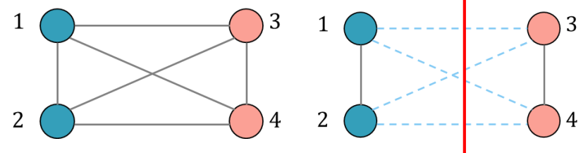
Taking a four-vertex example as shown in the figure below, we can observe that the “cut” method of dividing 1 and 2 into category A and 3 and 4 into category B will obtain the optimal solution to the problem: math: Z=4.

From the edge relationship, we can see that the adjacency matrix is:

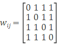
$\sum_{i<j,i \in V}\sum_{j \in V}w_{ij} = w_{12}+w_{13}+w_{14}+w_{23}+w_{24}+w_{34}$

$\sum_{i<j,i \in V}\sum_{j \in V}w_{ij}s_is_j = w_{12}s_1s_2+w_{13}s_1s_3+w_{14}s_1s_4+w_{23}s_2s_3+w_{24}s_2s_4+w_{34}s_3s_4$

When vertices 1 and 2 are in one group, and vertices 3 and 4 are in another group, $s_1=s_2=1, s_3=s_4=-1$ . Then the above formula becomes

$\sum_{i<j,i \in V}\sum_{j \in V}w_{ij}s_is_j = w_{12}-w_{13}-w_{14}-w_{23}-w_{24}+w_{34}$

At this time, the objective function is:

$max Z = (\sum_{i<j,i \in V}\sum_{j \in V}w_{ij}-\sum_{i<j,i \in V}\sum_{j \in V}w_{ij}s_is_j)/2= w_{13}+w_{14}+w_{23}+w_{24} = 4$

The maximum number of cuts is 4, which is consistent with the answer obtained through observation in the previous article.

Note that: math: w_{ij}is an input constant and does not affect the calculation of the model, so the above formula can be simplified to:

$min H = \sum_{i<j,i \in V}\sum_{j \in V}w_{ij}s_is_j$

Wherein, $H$ represents the Hamiltonian, $w$ is the input adjacency matrix, and the decision variable $s_i$ represents the classification of the vertex $i$ . The above formula is an Ising model for the maximum cut problem.

Modeling code#

Input Matrix#

import numpy as np
import kaiwu as kw

# Import the plotting library
import matplotlib.pyplot as plt

# invert input graph matrix
matrix = -np.array([
                [0, 1, 0, 1, 1, 0, 0, 1, 1, 0],
                [1, 0, 1, 0, 0, 1, 1, 1, 0, 0],
                [0, 1, 0, 1, 1, 0, 0, 0, 1, 0],
                [1, 0, 1, 0, 0, 1, 1, 0 ,1, 0],
                [1, 0, 1, 0, 0, 1, 0, 1, 0, 1],
                [0, 1, 0, 1, 1, 0, 0, 0, 1, 1],
                [0, 1, 0, 1, 0, 0, 0, 0, 0, 1],
                [1, 1, 0, 0, 1, 0, 0, 0, 1, 0],
                [1, 0, 1, 1, 0, 1, 0, 1, 0, 1],
                [0, 0, 0, 0, 1, 1, 1, 0, 1, 0]])

Calculations using the Classical Solver#

worker = kw.classical.SimulatedAnnealingOptimizer(initial_temperature=100,
                                                  alpha=0.99,
                                                  cutoff_temperature=0.001,
                                                  iterations_per_t=10,
                                                  size_limit=100)
output = worker.solve(matrix)

Output#

opt = kw.sampler.optimal_sampler(matrix, output, 0)
best = opt[0][0]
max_cut = (np.sum(-matrix)-np.dot(-matrix,best).dot(best))/4
print("The obtained max cut is "+str(max_cut)+".")

Beginner’s Tutorial 3 - Maximum Cut Problem

Contents