Beginner Tutorial 2-Traveling Salesman Problem#

What is the Traveling Salesman Problem#

The Traveling Salesman Problem (TSP) is a classic combinatorial optimization problem. The classic TSP can be described as: a salesman has to go to several cities to sell goods, The salesman starts from one city and needs to go through all the cities before returning to the starting point. How should he choose the route to make the total journey the shortest?

From the perspective of graph theory, the problem is essentially to find a Hamilton circuit with the minimum weight in a weighted completely undirected graph. Since the feasible solution to this problem is the full arrangement of all vertices, as the number of vertices increases, there will be a combinatorial explosion, and it is an NP-complete problem. Due to its wide application in transportation, circuit board design, and logistics distribution, scholars at home and abroad have conducted a lot of research on it. Early researchers used exact algorithms to solve this problem. Commonly used methods include: branch and bound method, linear programming method, dynamic programming method, etc. However, as the scale of the problem increases, the exact algorithm will become powerless. Therefore, In later studies, scholars at home and abroad focused on using approximate algorithms or heuristic algorithms, mainly genetic algorithms, simulated annealing methods, ant colony algorithms, taboo search algorithms, greedy algorithms, and neural networks. Today, the emergence of quantum computing provides a new way to solve this problem.

Analysis of the Traveling Salesman Problem#

The Nature of the Problem#

The traveling salesman problem is a bit like the shortest path problem, and then we will naturally think of using Dikstra’s algorithm to find: the shortest path from a certain city to all other cities, or if it is a real map, we can use the heuristic A star algorithm to quickly search for the shortest path from a certain city to another specified city. But if you think about it carefully, this problem is not as simple as that. It also requires finding the shortest tour path starting from a certain city, passing through other cities once and only once, and finally returning to the starting city.

In-depth analysis#

The traveling salesman problem is to find the tour route with the minimum cost from all the tour routes of the graph G. There are a total of $(n-1)!$ tour routes starting from the initial point, which is equal to the number of permutations of n-1 nodes excluding the initial node. Therefore, the traveling salesman problem is a permutation problem. Permutation problems are usually much more difficult to solve than subset selection problems. This is because there are $n!$ permutations of n objects and only $2^n$ subsets ( $n! > 2^n$ ). The algorithm that enumerates $(n-1)!$ tour routes and finds a tour route with the minimum cost obviously takes $O(n!)$ time to calculate.

So how to solve it? It’s easy for us to think of an exhaustive approach: Now suppose we want to visit 11 cities, starting from city 1 and returning to city 1. Obviously, after leaving city 1, we can immediately choose one of the remaining 10 cities to visit (all cities here are connected and always reachable, and the disconnected situation belongs to the decoration of personal special business, which is not considered in this case), so it is obvious that there are 10 choices here, and so on, there are 9 choices next time. The total number of optional routes is: 10!. That is to say, it takes 10! iterations of the for loop to find all the routes and then select the shortest one. If you only visit 10 cities (it takes 3628800 iterations), it may be okay, but visiting 100 cities (it takes 9.3326215443944*10^157 iterations) is simply a nightmare for classical computers! If there are more cities, the time overhead of calculation can be imagined!

More generally, if we want to visit n+1 cities, the total number of optional routes is $n!$ , and the time complexity is $O(n!)$ . From here we can also see that the time complexity of this algorithm is non-polynomial, and its high cost is obvious. So the key to the problem is not to find the shortest path between two cities, but to find the shortest tour path, in other words, to find a sequence of visiting cities in order.

Traveling Salesman Solution#

Traditional traveling salesman solution solutions mainly include:

TSP Traveling Salesman Problem - Brute Force Method (DFS)
TSP_Traveling Salesman Problem - Dynamic Programming
TSP Traveling Salesman Problem - Simulated Annealing Algorithm
TSP Traveling Salesman Problem - Genetic Algorithm
TSP Traveling Salesman Problem-Particle Swarm Optimization
TSP Traveling Salesman Problem - Neural Network

The traveling salesman problem is an NP-complete problem, and the exhaustive algorithm is not efficient. So how can we quickly find the order of priority through an algorithm with polynomial time complexity? The current mainstream method is to use some random and heuristic search algorithms, such as genetic algorithms, ant colony algorithms, simulated return algorithms, particle swarm algorithms, etc. However, these algorithms all have a disadvantage, that is, they may not necessarily find the optimal solution, but can only converge to (approximately approximate) the optimal solution and get a suboptimal solution, because they are essentially random algorithms, and most of them will screen solutions with a similar idea of ‘accept or discard with a certain probability’. The implementation ideas of each algorithm are different, but they also have more or less mutual reference. Some are related to random factors, some are related to initial states, some are related to random functions, and some are related to selection strategies.

Based on the above analysis, the solution to the TSP problem is roughly composed of the following two steps:

1. Calculate the shortest path between two cities: Use algorithms similar to Diikstra, Flord, and A-star to find the shortest route.

2. Calculate the shortest tour path: Use search algorithms such as genetic algorithms and ant colony algorithms to find the order of tour visits. One thing that needs to be explained about 1 is that in real life, our map is often not a complete graph, but an incomplete graph. Some nodes are even just road forks, not city nodes. The difference between a complete graph and an incomplete graph is as follows.

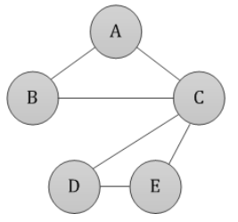
Complete and Incomplete Graphs#

Complete graph: There is a direct route between two cities, and this route does not need to pass through other nodes in the middle;

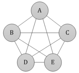
Incomplete graph: Occasionally, a route between two cities needs to pass through other intermediate nodes.

Applying quantum computing to solve the traveling salesman problem#

1. Variable definition#

Given a weighted connection graph ， is the set of nodes， is the set of edges.
We use the distance matrix to represent, When there is no edge between two points, the weight value is.
let ，represents the number of nodes.
letmeans pointis visited at thepoint, otherwise。
where, 。

2. Constraint handling#

First of all, we need that for each $u$ , there is only one sequence $j$ , then there is:

$\sum_{j=0}^{N-1}x_{u,j}=1, \quad u \in 0...N-1$

Secondly, we need that for each sequence $j$ , there is only one point $u$ , then there is:

$\sum_{u=0}^{N-1}x_{u,j}=1, \quad j \in 0...N-1$

Write the above two constraints in QUBO form, as follows:

$A \sum_{u=0}^{N-1} (\sum_{j=0}^{N-1}x_{u,j}-1)^2 + A \sum_{j=0}^{N-1} (\sum_{u=0}^{N-1}x_{u,j}-1)^2$

For $(u,v)\notin E$ , we want $u$ , $v$ If discontinuous occurrences occur at positions $j$ and $j+1$ , then:

$A \sum_{(u,v)\notin E}(\sum_{j=0}^{N-2}x_{u,j}x_{v,j+1} + x_{u,N-1}x_{v,0})$

3. QUBO model construction#

In this way, from the above QUBO, we can construct a model of a path that traverses all points (also called a Hamilton ring):

$H_A = A \sum_{u=0}^{N-1} (\sum_{j=0}^{N-1}x_{u,j}-1)^2 + A \sum_{j=0}^{N-1} (\sum_{u=0}^{N-1}x_{u,j}-1)^2 + A \sum_{(u,v)\notin E}(\sum_{j=0}^{N-2}x_{u,j}x_{v,j+1} + x_{u,N-1}x_{v,0})$

However, for the traveling salesman problem, based on this, we want to obtain the shortest one of the above paths. Let $w_{u,v}$ be the edge $(u,v)$ The weight is:

$H_B = B \sum_{(u,v)\in E}w_{u,v}(\sum_{j=0}^{N-2}x_{u,j}x_{v,j+1} + x_{u,N-1}x_{v,0})$

Adding two QUBO expressions yields the final optimized model:

$H = H_A + H_B$

The optimization objective is to find the minimum value of H

4. Use Solver to solve QuboModel directly#

Load dependency packages

# Import numpy and kaiwu
import numpy as np
import pandas as pd
import kaiwu as kw

Load graph data and perform preprocessing

# Import distance matrix
w = np.array([[ 0, 13, 11, 16,  8],
              [13,  0,  7, 14,  9],
              [11,  7,  0, 10,  9],
              [16, 14, 10,  0, 12],
              [ 8,  9,  9, 12,  0]])

# Get the number of nodes
n = w.shape[0]

# Create qubo variable matrix
x = kw.qubo.ndarray((n, n), "x", kw.qubo.Binary)

# Get sets of edge and non-edge pairs
edges = [(u, v) for u in range(n) for v in range(n) if w[u, v] != 0]
no_edges = [(u, v) for u in range(n) for v in range(n) if w[u, v] == 0]

Load constraints and construct objective function

def is_edge_used(x, u, v):
    return kw.qubo.quicksum([x[u, j] * x[v, j + 1] for j in range(-1, n - 1)])

qubo_model = kw.qubo.QuboModel()
# TSP path cost
qubo_model.set_objective(kw.qubo.quicksum([w[u, v] * is_edge_used(x, u, v) for u, v in edges]))

# Node constraint: Each node must belong to exactly one position
qubo_model.add_constraint(x.sum(axis=0) == 1, "sequence_cons", penalty=20)

# Position constraint: Each position can have only one node
qubo_model.add_constraint(x.sum(axis=1) == 1, "node_cons", penalty=20)

# Edge constraint: Pairs without edges cannot appear in the path
qubo_model.add_constraint(kw.qubo.quicksum([is_edge_used(x, u, v) for u, v in no_edges]),
    "connect_cons", penalty=20)

5. Calculations using the Classical Solver#

This problem has three hard constraints (point constraints, position constraints and edge constraints). The value of the hard constraints must be strictly $0$ Only to form a legal path. Sometimes the hard constraints of the CPQC simulator are not $0$ , so we find a solution that satisfies the hard constraints in the neighborhood of the CPQC simulator result by running a tabu search on the result.

# Perform calculation using SA optimizer
solver = kw.solver.SimpleSolver(kw.classical.SimulatedAnnealingOptimizer(initial_temperature=100,
                                                                         alpha=0.99,
                                                                         cutoff_temperature=0.001,
                                                                         iterations_per_t=10,
                                                                         size_limit=100))

sol_dict, qubo_val = solver.solve_qubo(qubo_model)

6. Calculate the final path#

Above we have obtained the spin result, which needs to be converted into the value of the original variable before we can further give the path to be obtained. We use the get_val module for conversion.

# Check the hard constraints for validity and path length
unsatisfied_count, res_dict = qubo_model.verify_constraint(sol_dict)
print("unsatisfied constraint: ", unsatisfied_count)
print("value of constraint term", res_dict)

# Calculate the path length using path_cost
path_val = kw.qubo.get_val(qubo_model.objective, sol_dict)
print('path_cost: {}'.format(path_val))

unsatisfied constraint:  0
value of constraint term {'sequence_cons(0,)': 0.0, 'sequence_cons(1,)': 0.0, 'sequence_cons(2,)': 0.0, 'sequence_cons(3,)': 0.0, 'sequence_cons(4,)': 0.0, 'node_cons(0,)': 0.0, 'node_cons(1,)': 0.0, 'node_cons(2,)': 0.0, 'node_cons(3,)': 0.0, 'node_cons(4,)': 0.0, 'connect_cons': 0.0}
path_cost: 50.0

Above we have obtained the legality and length of the path. Next we restore the value of the $x$ variable and obtain the path.

if unsatisfied_count == 0:
    print('valid path')

    # Get the numerical value matrix of x
    x_val = kw.qubo.get_array_val(x, sol_dict)
    # Find the indices of non-zero items
    nonzero_index = np.array(np.nonzero(x_val.T))[1]
    # Print the path order
    print(nonzero_index)
else:
    print('invalid path')

valid path
[0 1 2 3 4]

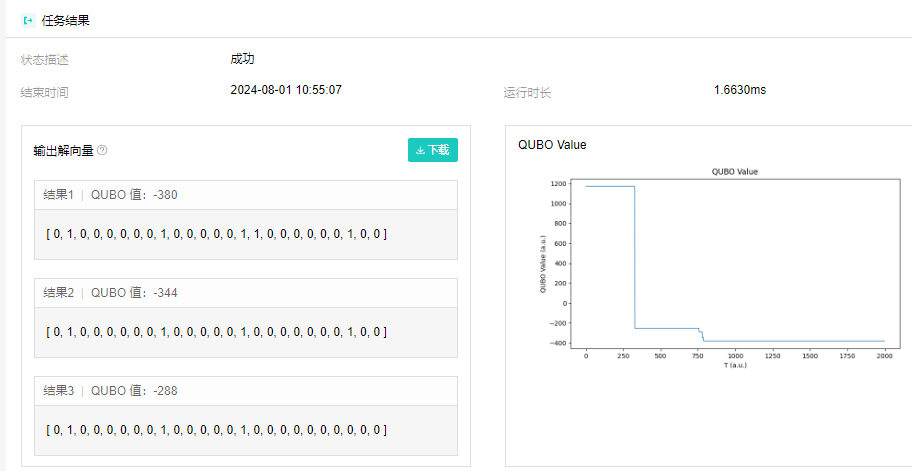
7. Using CPQC for calculations#

Using the Bose quantum cloud platform to call a coherent Ising machine to solve the TSP problem, the results obtained are shown in the following figure. The result has been verified to be the same as the above method, with a time consumption of approximately 1.66ms.

../_images/TSP_cloundplatform_cim_result.png

Beginner Tutorial 2-Traveling Salesman Problem

Contents